Volume Rendering, Maximum Intensity Projection and Isosurfaces
|
Introduction
The dataset consists of the human head CT scan as well as a computational fluid dynamics simulation of a delta wing aircraft in a critical flight configuration. We visualize the data using isosurfacing and volume rendering. We also design transfer functions for both color mapping the salient regions and for opacity. In the last part, we design a multidimensional transfer function where we use both the scalar value and the gradient magnitude to control the opacity. We make a comparison of volume rendering and isosurfacing where the conditions/visualization parameters are controlled in order to make a fair visual comparison between the two approaches. In part 4, we apply Maximum Intensity Projection where the volume rendering integral is reduced to measuring the maximum scalar value along each ray. We also apply volume clipping in order to identify regions of interest which are difficult to see otherwise (i.e., white matter). Further, we apply various color maps to the Maximum Intensity Projection in order to separate the regions of higher density more clearly. In part 5, we design a few multi-dimensional transfer functions for both the Head CT Dataset and the Lambda2 Wing Dataset. We also apply various clipping planes and other techniques to extract interesting features in order to illustrate the significance of the multi-dimensional transfer functions. We have also provided the ability to take multiple screenshots by pressing the 'm' key. The resolution of the images is double the current size of the rendered window and are saved in the working directory. |
Part 1: Salient Isovalues The first task is to extract the most significant isovalues that correspond to boundaries within both the head CT dataset and the computational fluid dynamics simulation of a delta wing aircraft. The surfaces of interest within the head CT dataset are the skin, tissue, bones, and white matter. As for the fluid dynamics dataset we are interested in discovering the vortices (i.e., spinning, turbulent, flow of fluid) present on both sides of the wing. For both datasets, we used a slider to explore the structures pertaining to selected isovalues and attempted to identify visually the boundaries of where the gradient magnitude changes significantly between isovalues as these regions are most likely to pertain to boundaries. The gradient magnitudes are commonly used to evaluate and detect boundaries. Capturing the boundaries allows us to characterize them using transfer functions for color and opacity. More specifically, the design of transfer functions relies on the notion of boundaries. Further, the boundaries can be identified by defining derivatives with respect to the direction of the normal. We might then project the gradient onto the direction/normal and from this the boundary should show up as a remarkable signature in that reference frame. |
Part 1.1: Salient Isovalues for the Head CT Dataset In the CT head dataset we used a classification color map where particular isovalues correspond to skin, tissue, bone, and white matter. The isovalues we discovered for each boundary/isosurface are {700->Skin, 1050->Tissue, 1150->Bone, 1300->White Matter} and each isovalue is also mapped to an opacity {700->0.05, 1050->0.3, 1150->0.85, 1300->1.00}. We are not able to clearly visualize the white matter as shown. We even attempted to capture the white matter by applying clipping planes. We suspect that the white matter pertains is at a lower density than bone, but to properly visualize it we must first remove the skull. The tissue is a bit difficult to capture as well since the tissue is not captured with only one isovalues (i.e., captured with many isosurfaces). The rest of the boundaries are straight-forward to detect as bones and skin are continuous for the most part along one isosurface. The opacities were selected such that all surfaces are able to be clearly visualized. Therefore skin is more transparent than tissue which is more transparent than bone and so forth. A realistic color classification map is also applied. 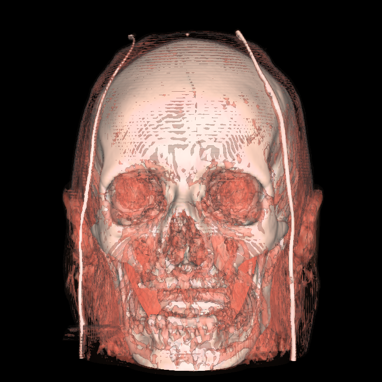   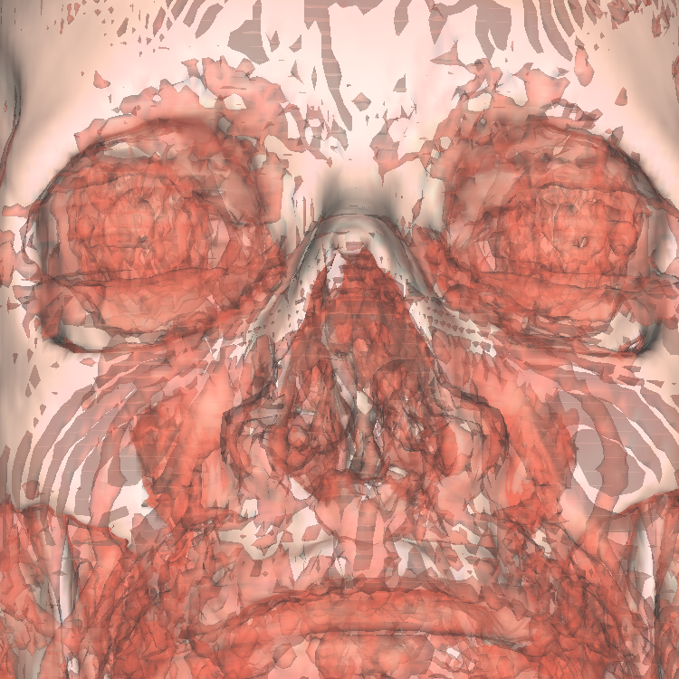 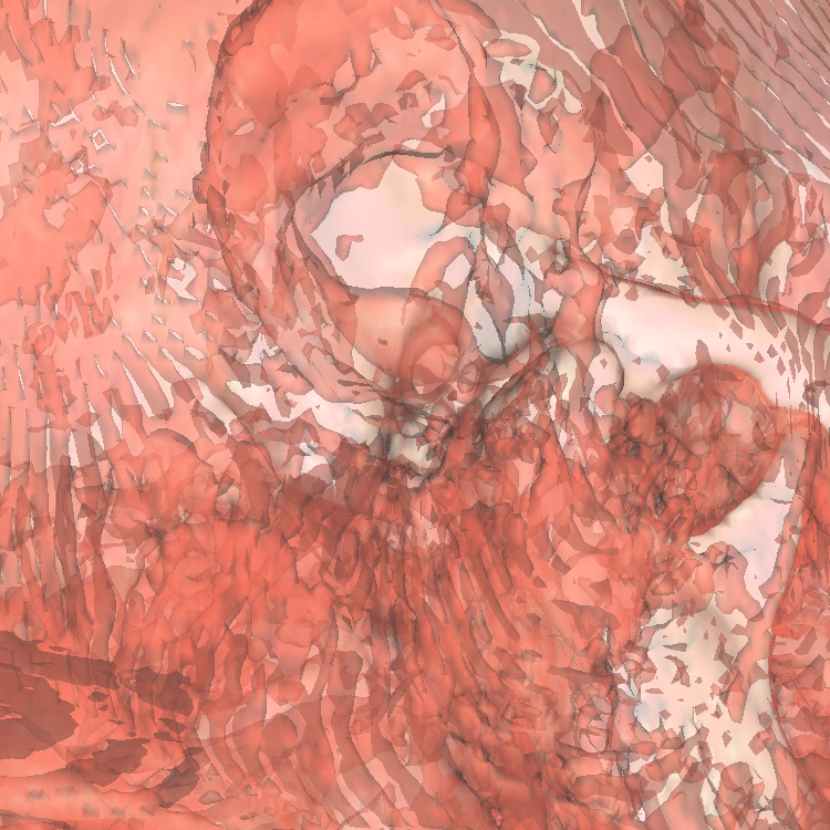  |
|
We also tried eliminating most of the oscillating tissue in order to see more clearly the bone structures and perhaps tissues that lie around the boundary regions. This is accomplished by simply making the skin (700-800) and tissue (1050) extremely transparent. |
Part 1.2: Salient Isovalues for the Delta Wing Aircraft Simulation It is very difficult and insufficient to strictly use isosurfaces to capture or detect the vortices in a typical aircraft flow. This is related to the premise that vortices are not strictly isolated from each other. We find that the most suitable vortice visualization is most likely found at the boundaries; rather than in between. However, we are still able to capture many of the interesting surfaces. We first discuss our approach to capturing the structures and then discuss our specific design and settings for opacity. First, we had to convert the dataset to unsigned short to be able to visualize it appropriately. Below we show the evolution of the structures as we increase the isovalue from 10000 to 50000. This allows us to see that as the isovalues increase more of the inner vortices are clearly shown and we also notice that as the isovalue increases the vortices shrink in diameter. We also notice that throughout this range, the vortices are not independent of one another (i.e., we are inbetween the boundaries of the structure). 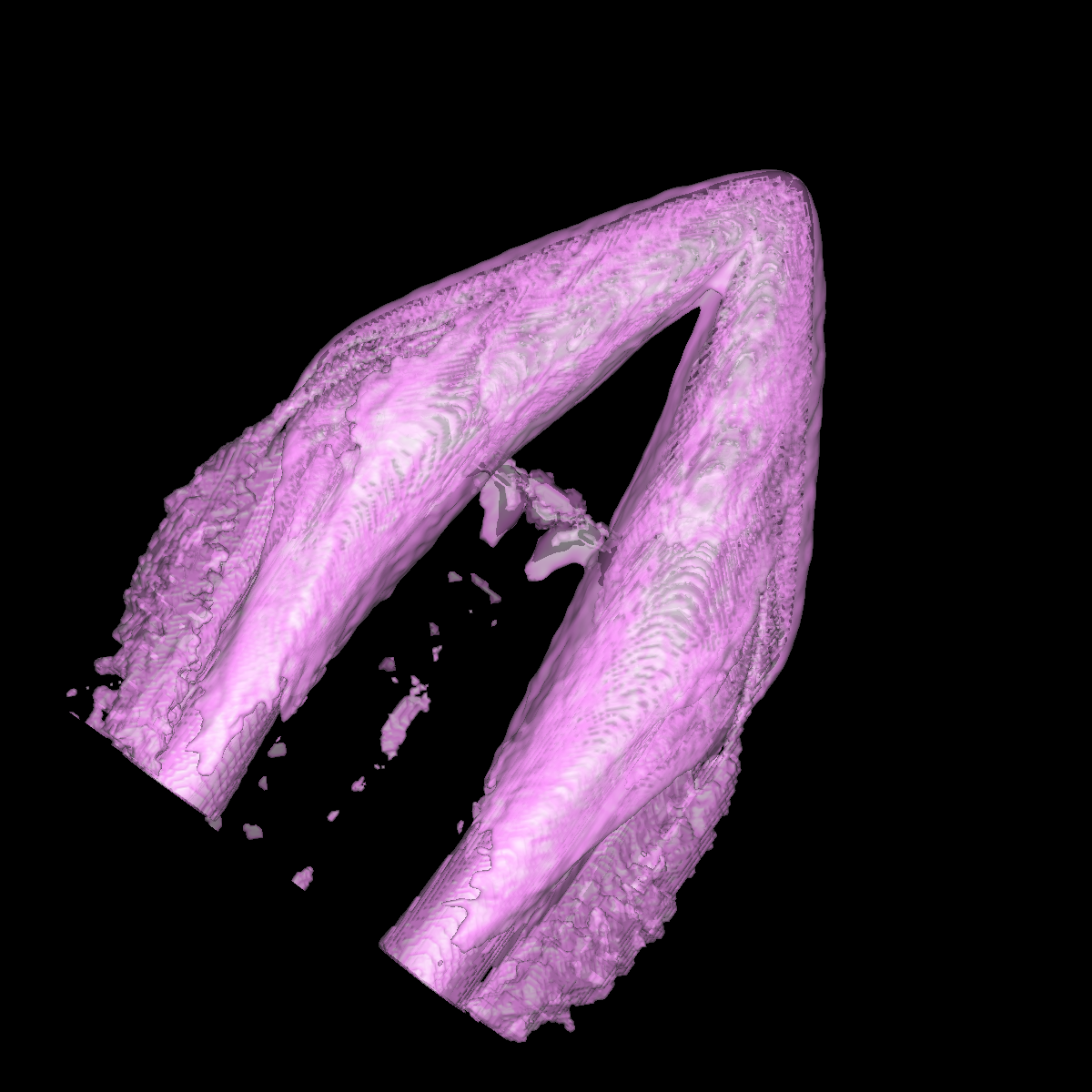 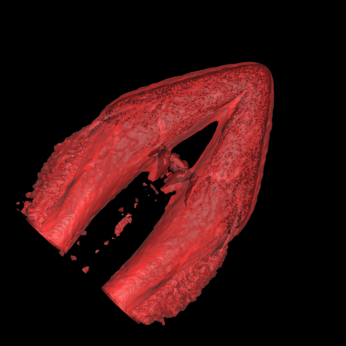 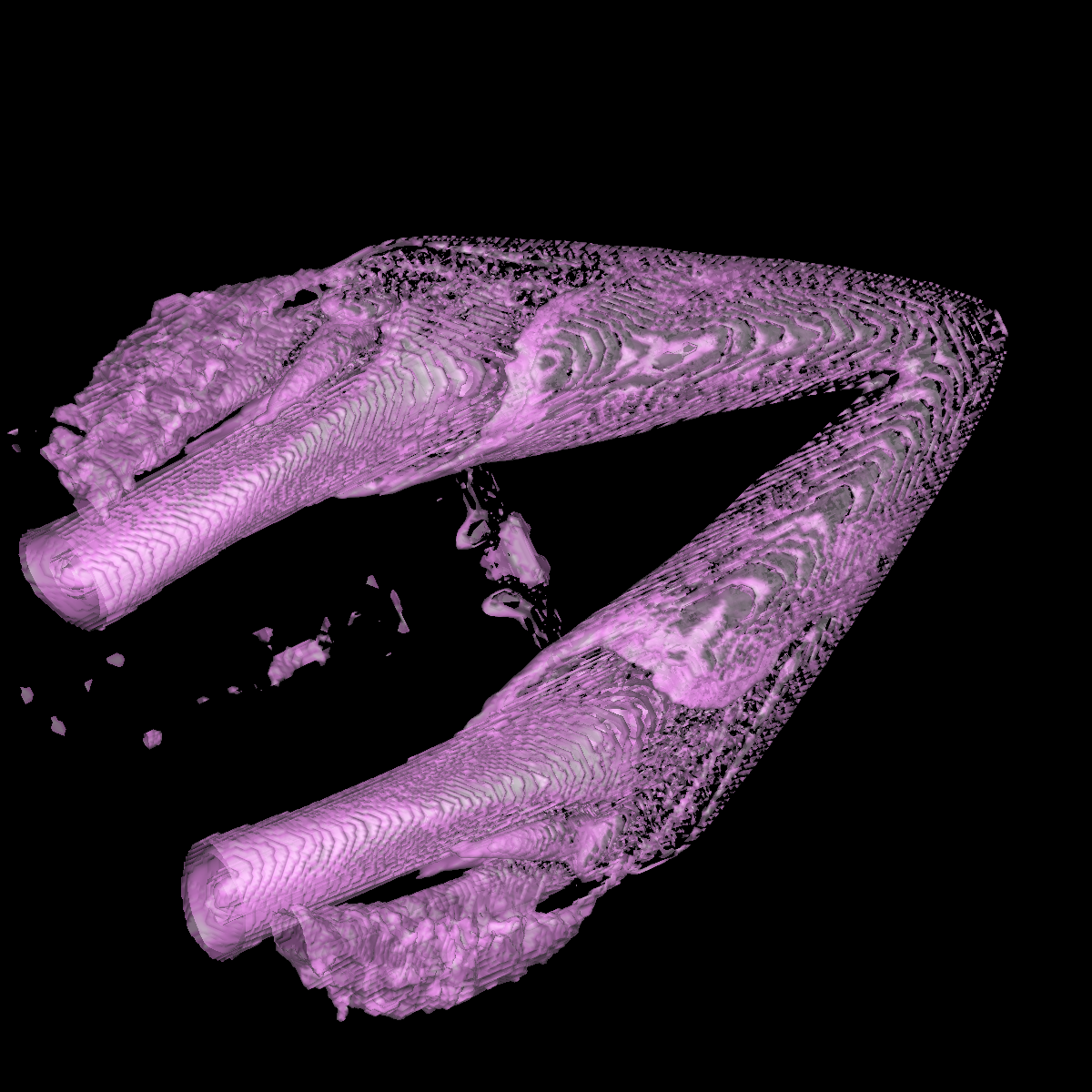 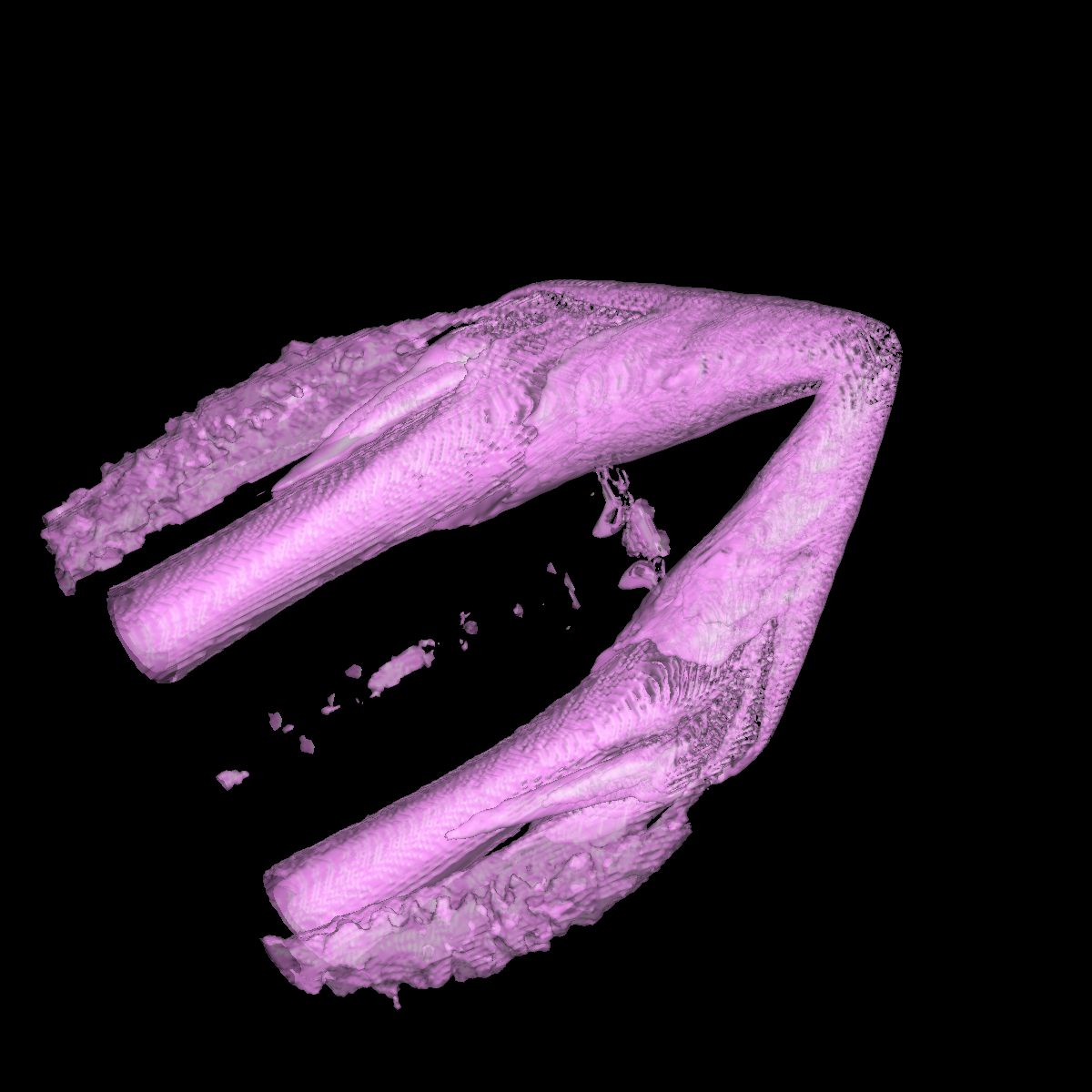 |
We found four main structures/boundaries within the computational fluid dynamics simulation of the delta wing aircraft. A classification color map is used to idenitfy the structures. In the original lambda2 dataset with negative values, we found that the interesting features corresponded to low negative values. However, the dataset was converted to unsigned short and now the interesting values mainly correspond to larger values. We also found that some interesting features are captured independently and for the lambda2 dataset in particular (since things are highly embedded and not as simple as the head) the details and ability to appropriately capture these features depend on the opacity and colors of the other structures. In this respect, we designed many visualizations and show a few of them below. The wing is much more difficult to visualize then the head CT scan datasets as the boundaries are much more well defined. The wing most likely requires feature extraction and data manipulation as a preprocessing step to visualizing some of the vortices and interesting features in general. The structures were identified by finding the boundaries using the slider and information about vortices/fluid dynamics. A boundary is defined as a region with high gradient magnitude. Alternatively, we could have used this intuition to identify boundaries in a semi-automatic fashion. We defined the following four isosurfaces at the isovalues {2000, 10000, 35000, 50000} with the corresponding opacities {0.15, 0.20, 0.50, 0.50} and colors {blue, green, white, red}. The vortices have somewhat distinct boundaries where smaller vortices are inside one another as shown in the figures below. In particular, we choose an isovalue of 10000 and find the main vortice where multiple tubes/spirals are embedded within one another. We chose a transparency of 0.20 in order to clearly see all the tubings inside. The isosurface at 2000 corresponds to the larger spiral/tube on the outside. One interesting vortice is captured at 35000 and the other two main ones are captured at 50000. The isosurface at 50000 (red) clearly shows the spiral. We believe these three main vortices correspond to the vortices shown in the drawing provides in the project description. To highlight these three vortices, we attempted to find their boundaries in order to assign each one a specific color. The most difficult vortice to see is the smallest one forming from the red isosurface. Since the two isosurfaces at 35000 and 50000 are most independent from one another, we assigned them the same transparency. We chose 0.5 to allow us to see other rings/spiral within and around these structures.   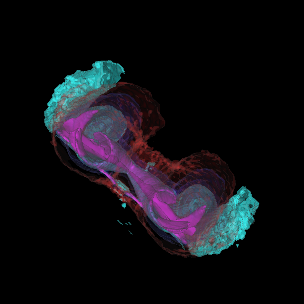 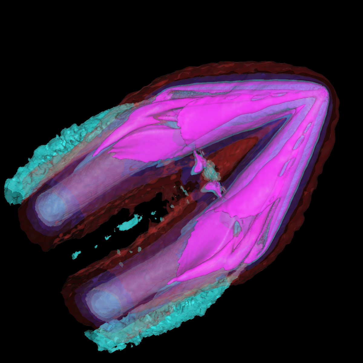 |
We have also tried to capture substructures using one more isosurface at isovalue 30000 (i.e., represented as green). From this visualization, the vortices from the tip of the wing are now represented as green while the larger vortices remain cyan. The vortices are a fuzzy structure and is difficult to capture using only a few isosurfaces. More specifically, if interested in details and visualizing the entire vortices at all layers, then volume rendering is probably the best choice. However, if interested in simply identifying the underlying structure and position then isosurfaces might be a better choice. 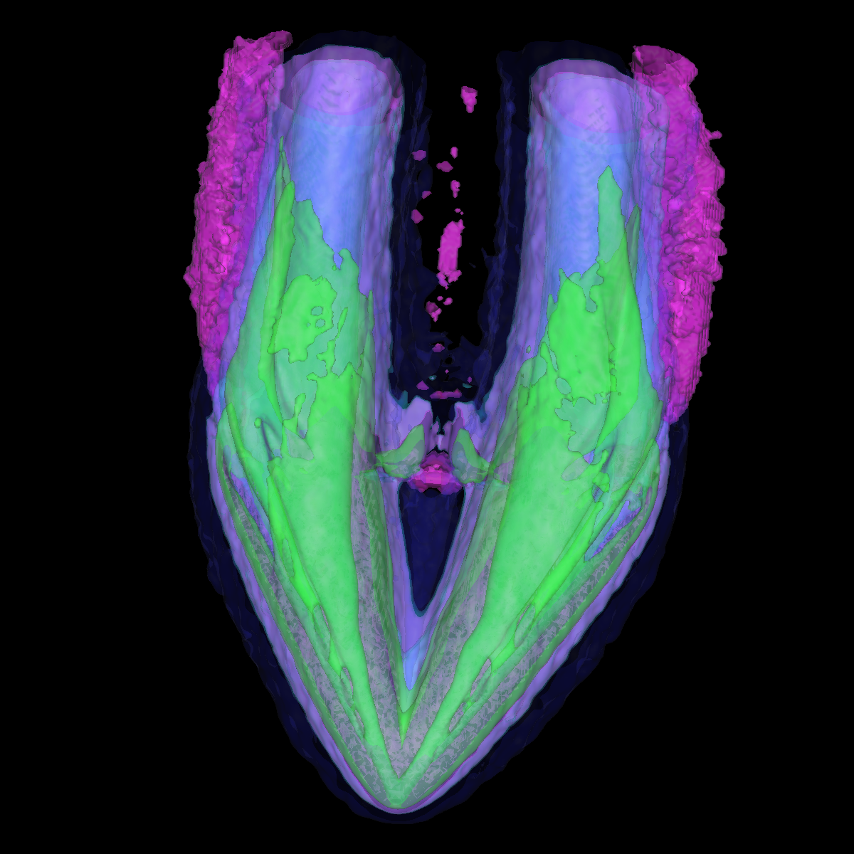 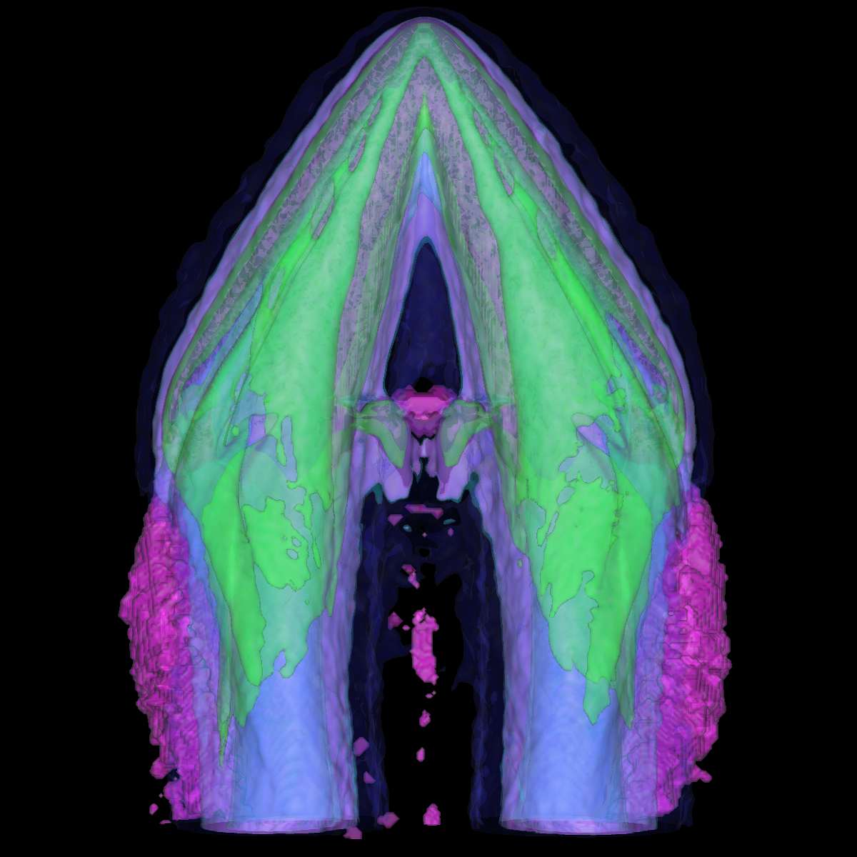   |
We also attempt to capture the spirals/vortices inside the larger structure.  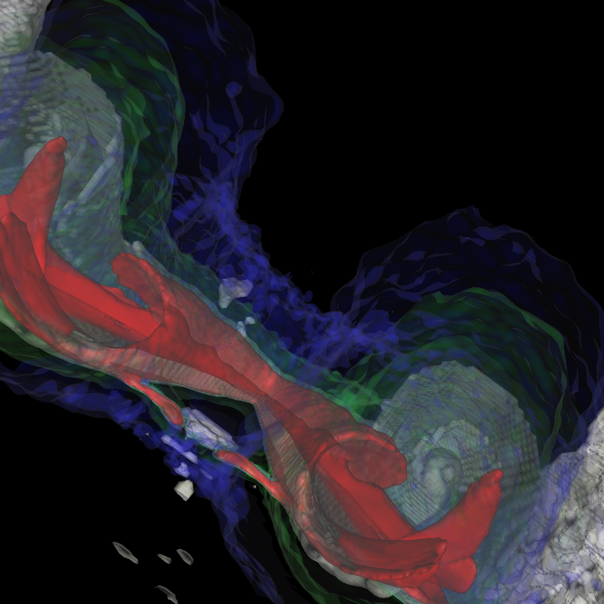 |
 |
Part 2: Designing Transfer Functions We apply ray casting to render the volumes and design color and opacity transfer functions to emphasize the significant boundaries/surfaces. We apply a classification color map and experiment with many opacity transfer functions for each dataset as shown below. Trilinear interpolation with a small sampling distance (i.e., 0.1) along each ray is used for rendering. The objective of the transfer functions is to show as much detail as possible of the internal structures. |
Part 2.1: Head CT Dataset For the head we show three different opacity transfer functions and describe the advantages and disadvantages of each approach. In particular, the volume rendering strictly using a scalar value to map opacity values fails as the flat surfaces such as the tissue dominate the rendering making it difficult to see other interesting features that are beyond the tissues. In essence, we attempt to design an opacity transfer function that counters this problems by making tissues more transparent. Nevertheless, we lose a lot of information and details in the process. As a first attempt, we defined the following opacity transfer function {700->0.0, 800->0.1, 1050->0.2, 1150->0.5, 1300->1.00}. This opacity transfer function is most similar to the opacity values we used for isosurfacing. However, this transfer function when applied for volume rendering fails to capture internal structures or even different tissue types. This is an artifact of the tissue dominating the feature space as the values corresponding to the tissues oscillates making it very difficult to view internal structures. 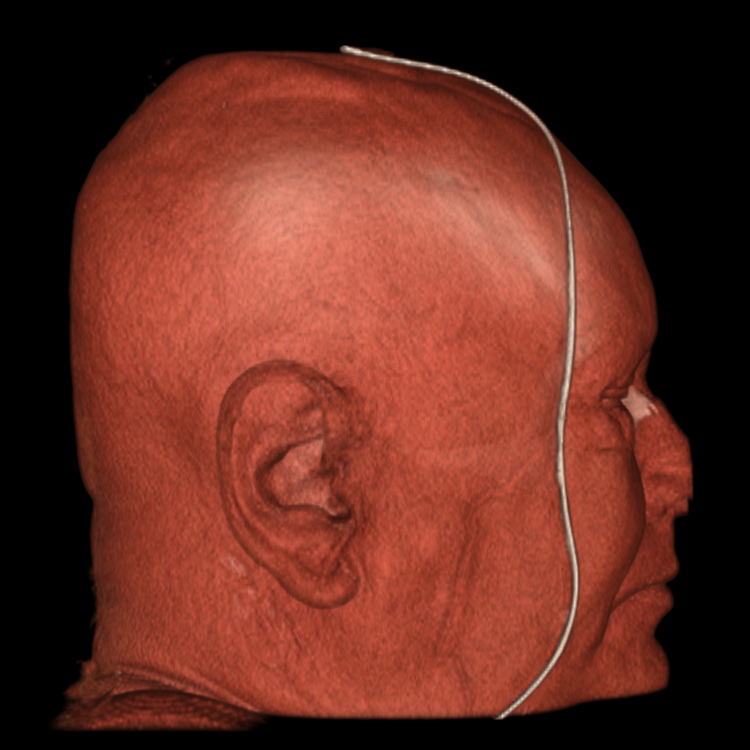 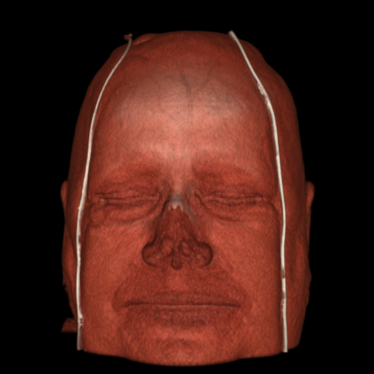 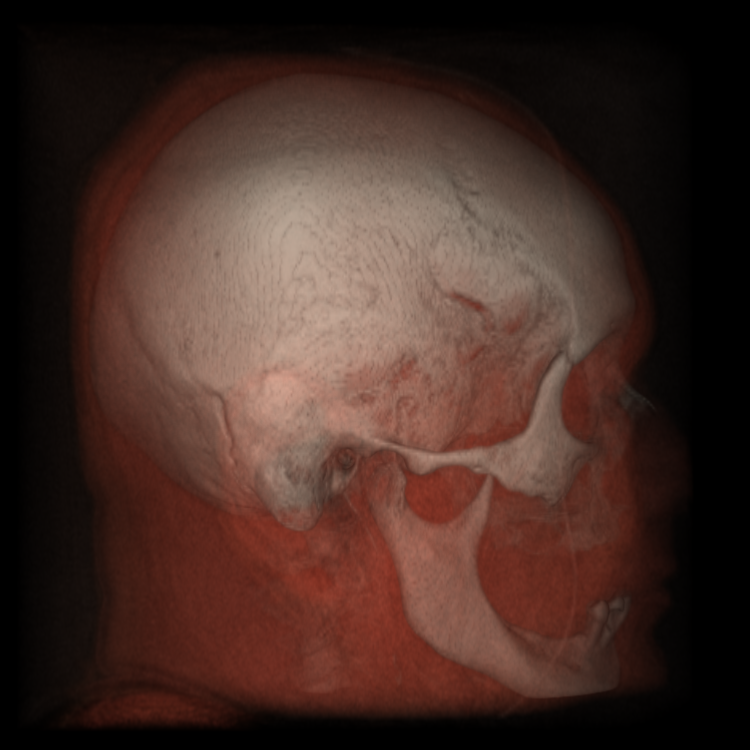 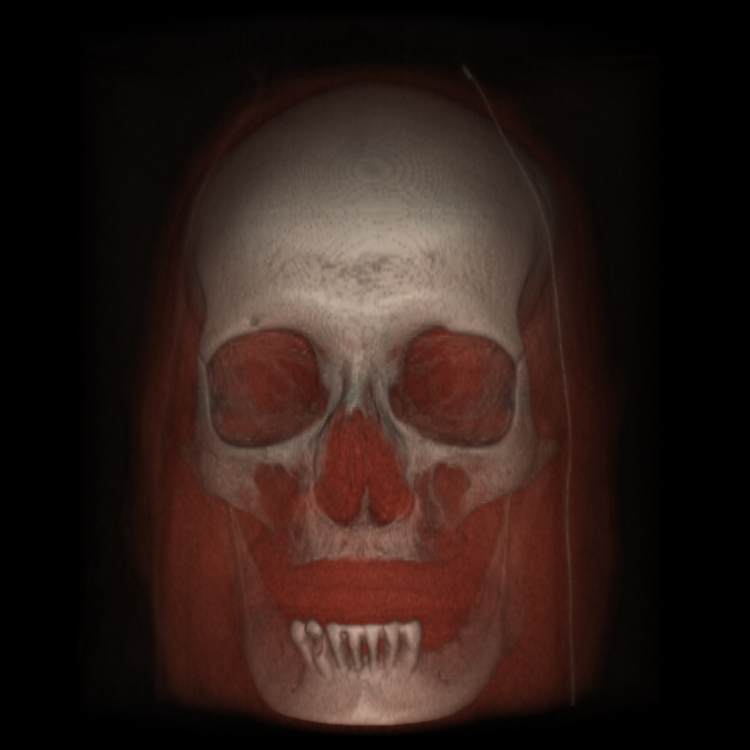  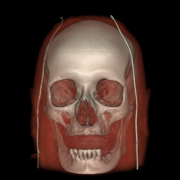 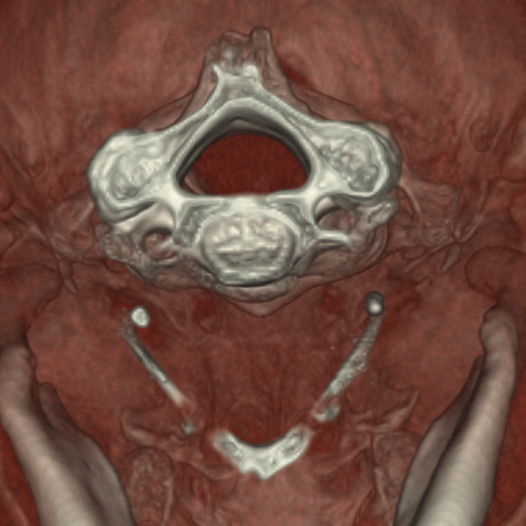  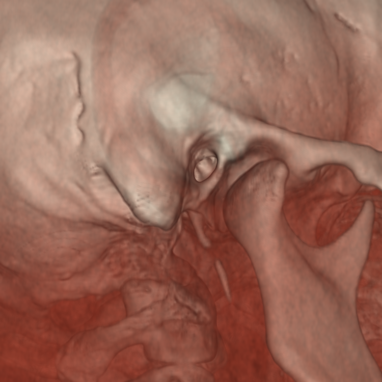 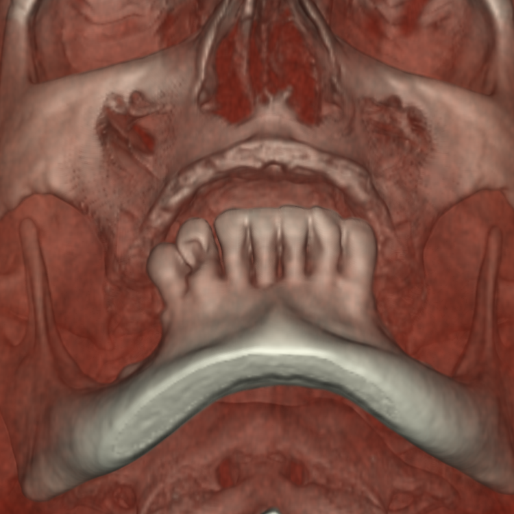 |
Part 2.2: Delta Wing Aircraft Simulation We design multiple transfer functions in order to visualize the vortices of the delta wing aircraft. As a first attempt, we designed the following opacity transfer function {1900-> 0, 2000->0.005, 10000->0.005, 35000->0.02, 50000->0.5}. In this function, we clamp any value under 1900 to be completly transparent. This function follows from the intuition observed with the isosurfaces. However, in volume rendering we used extremely small opacity values compared to the isosurfaces. This is due to the fact that volume rendering can be viewed as consisting of an infinite amount of surfaces and to see through these surfaces they must all be very transparent. This problem was also experienced with the tissues. We used the same classification color map. This transfer function allows us to visualize most of the interesting features. In the renderings below, we can even see smaller spirals that were not explictly captured in the isosurfaces. We chose the second transfer function to use as for comparision in part 3. Although, this is not necessarily the best, it is difficult to capture all the interesting features in one volume rendering without reducing the significance of others. This is an inherent problem with the structure of the lambda2 volume. Nevertheless, the other transfer functions could have been used as well and are interesting as well, especially the third and fourth transfer functions.  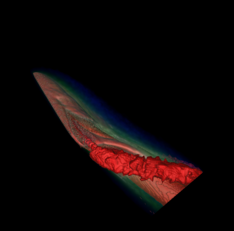 |
The second transfer function is defined as {1999->0, 2000->0.005, 10000->0.005, 10001->0, 34999->0, 35000->0.02, 50000->0.50} and used the following classification color map {2000->red, 10000->blue, 35000->cyan, 50000->pink}. Notice that in the opacity function we have clamped the values from [0,1999] and [10001,34999] to be fully transparent. The opacity function allows us to clearly visualize the smaller vortice and the color map also makes it stand out from the larger vortices.   In the image on the right we are able to see spirals highlighted in both pink and blue extending from the larger vortice.  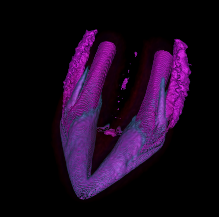 |
Another significant transfer function we found is defined as {20000->0, 25000->0.05, 25001->0, 35000->0, 60000->0.20} and uses the following classification color map {25000->pink, 50000->cyan, 60000->green}. We have again clamped the values, but this time more significantly in order to highlight what we believe to be the most significant vortices. We allow values in the range [20000,25000] in order to highlight the larger vortice. The smaller vortices inside this larger one are shown as cyan. We are able to again find the smaller vortice assigned green. We believe this is one the most useful transfer functions we designed (as it captures the most significant features) without applying a semi-automatic technique or using the gradient magnitude. 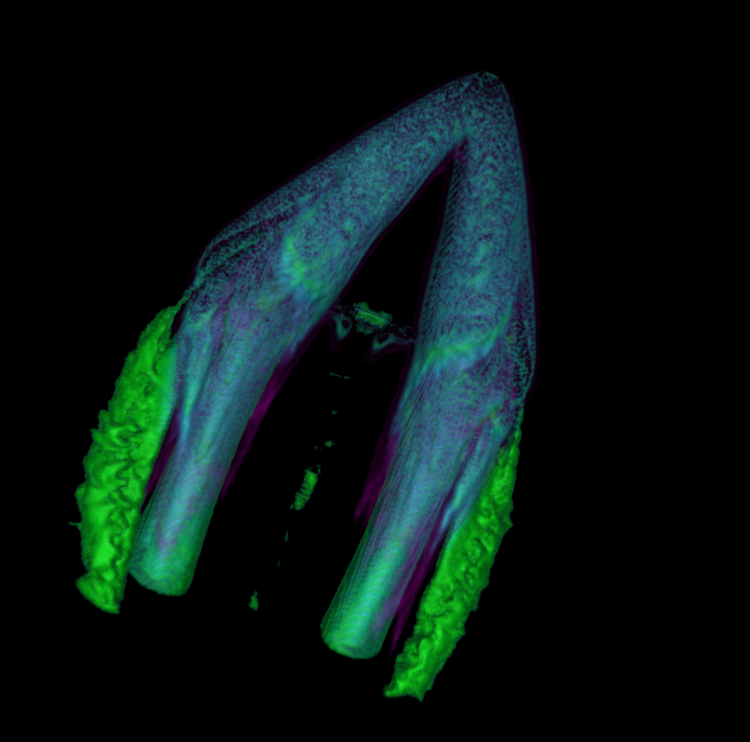  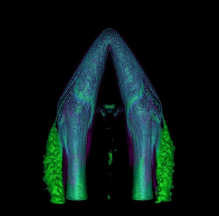  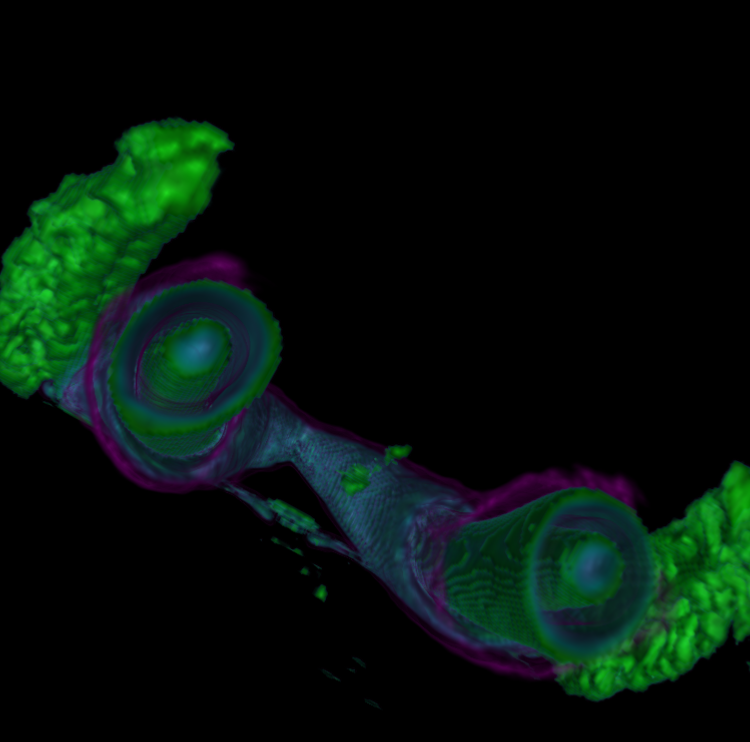 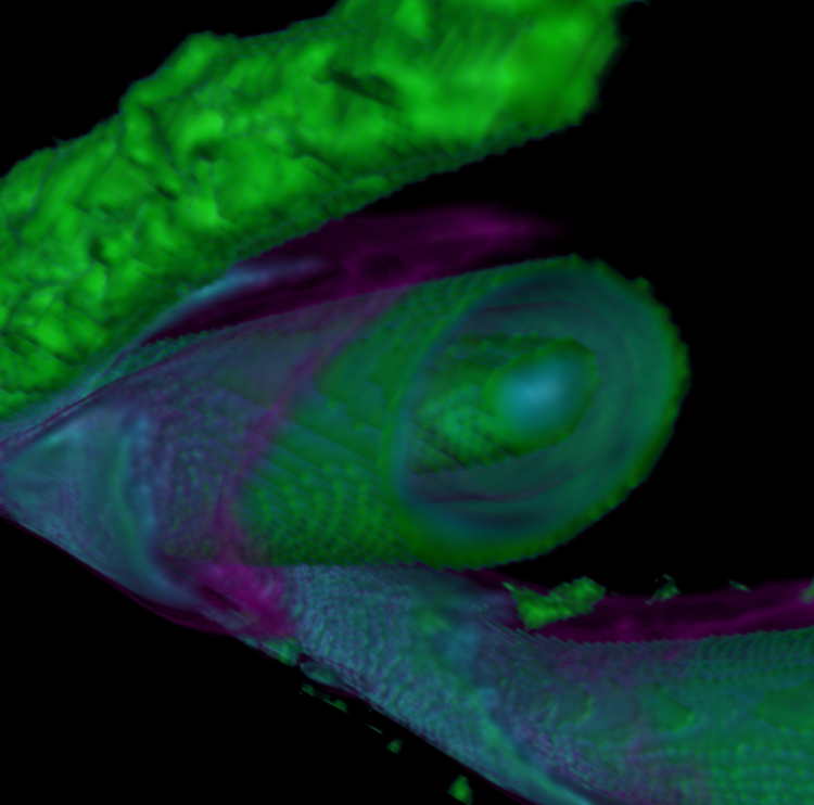 |
The last transfer function is designed to visualize the internal vortices of the larger vortice. For this purpose, we define the transfer function {34999->0, 35000->0.02, 50000->0.10, 60000->0.20} with the color map {35000->cyan, 50000->pink, 55000->green, 60000->red}. In this visualization we restrict our attention to only the internal vortices in the range [35000,end]. We are able to clearly see multiple vortices of varying sizes. As with the larger vortices, the smaller ones are not captured by a single or even a large range of values. Therefore it is extremely difficult to map these individual vortices to any specific color without also incorporating larger structures. We posit that isosurfaces are more suitable for capturing these structures. Each of the proposed transfer functions capture unique structures. It is extremely difficult to capture all these interesting structures in just one visualization by only using the scalar value to map the opacities. Perhaps using a combination of the gradient magnitude and scalar value will allow us to differentiate these structures from one another.  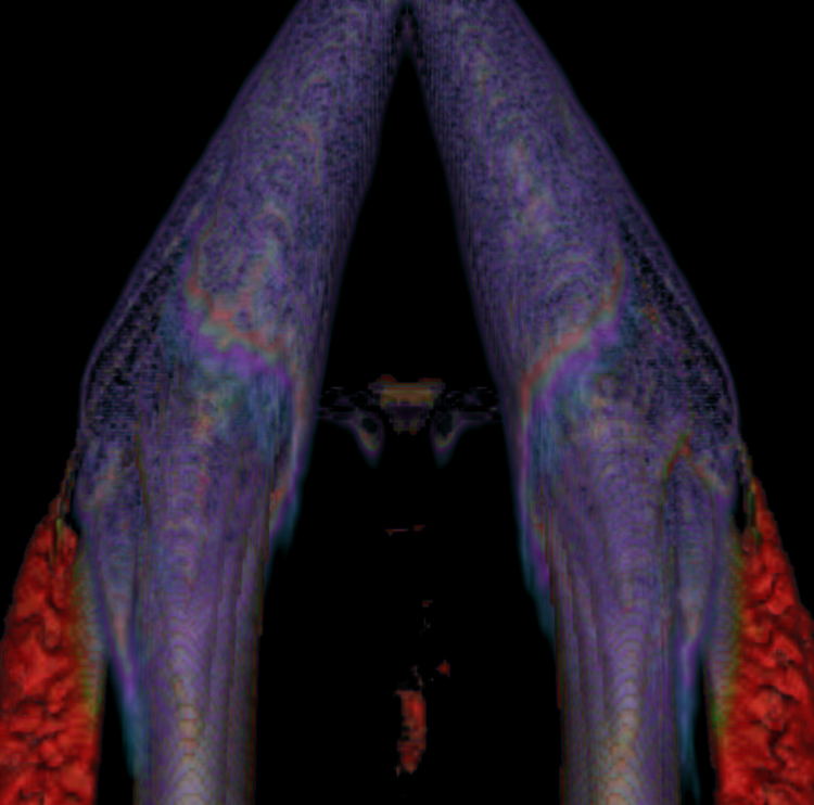  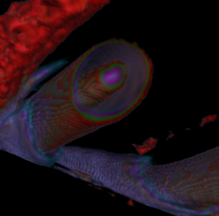 |
Part 2.2: Other Transfer Functions for the Delta Wing Aircraft Simulation We have also provided renderings of a few of the other transfer functions we designed. We believe the combination of these images provides a lot of intuition of the underlying structures. 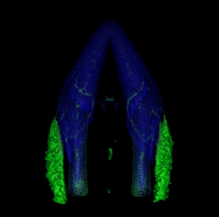 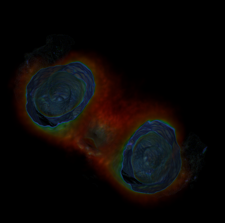  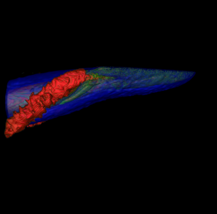 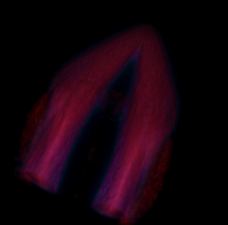 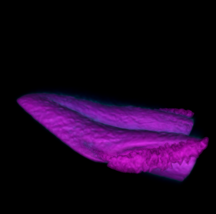 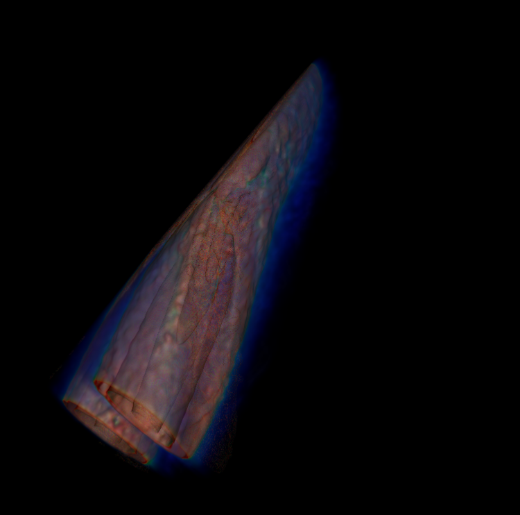     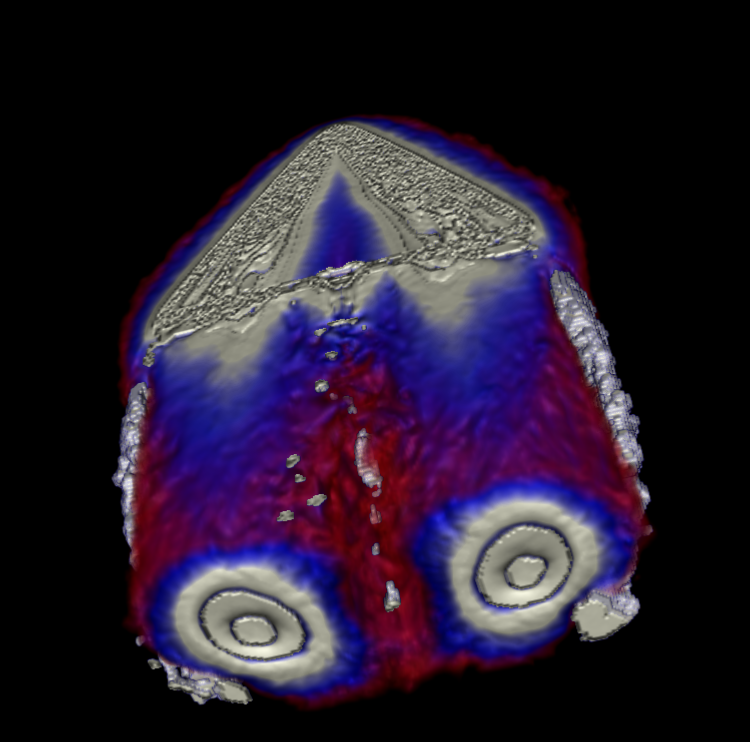 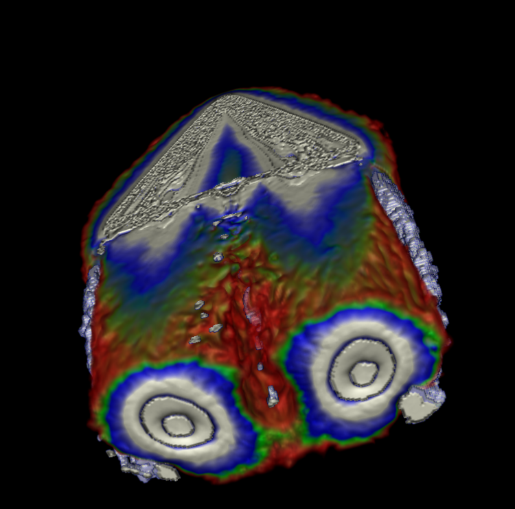 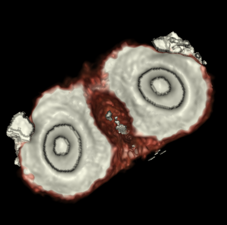 |
Part 3: Volume Rendering vs. Isosurfacing We compare volume rendering to isosurfacing using identical experimental conditions to objectively evaluate both approaches. There are significant differences between the two approaches and both have advantages and disadvantages. The use of either volume rendering or isosurfaces intrinsically depends on the application or task at hand and perhaps the resources as well. One disadvantage of isosurfaces is that an isosurface must be explictly defined for each structure whereas in volume rendering the majority of the structures can be captured with very little effort. Once the structures are discovered, a transfer function can be designed to refine and highlight significant aspects of each structure. The most immediate drawback with isosurfaces is the significant computational cost compared to volume rendering (i.e., at least with these particular datasets). Perhaps this is not an issue if the best hardware is used for rendering the visualizations. For instance, on my new laptop with an integrated video card the isosurfacing rendering can take up to 5 minutes whereas the volumes are rendered within seconds. We highlight significant advantages and disadvantages by comparing the interesting features rendered with each. A few of the main general advantages and disadvantages found in our experiments are listed below:
|
Part 3.1: Head CT Dataset For the Head CT dataset, we find that volume rendering provides the most detail and information for doctors and researchers. However, there are still a few features that are captured best by isosurfaces as shown. The effectiveness of the techniques will therefore depend on the goal, task, or the particular structure that is the target of the visualization. For the isosurfaces and volume renderings using ray casting we applied the precise transfer functions for color and opacity as discussed previously. |
Part 3.1.1: Front-view of the head The volume rendering captures significant details with respect to the bones whereas the isosurfacing misses these details and captures a more global view of the bones. However, the isosurfacing captures more specific details in the muscles/tissues while the volume rendering assigns a somewhat uniform value to these specific tissues. The volume rendering does allow us to see very clearly other interesting tissues, but it explictly misses the tissues seen in the isosurface rendering. However, if we were explictly interested in capturing these tissues seen in the isosurfacing then we could do this by restricting the volume rendering to target these tissues and conversely with respect to isosurfacing.  |
Part 3.1.2: Spinal cord and jaw The volume rendering captures a very detailed view of the spinal cord and bones surrounding it. The advantage of the volume rendering here is the ability to explictly represent regions between where the bone starts and finishes whereas isosurfacing simply creates a surface around the bone/spinal cord and details inside are not clearly defined. More generally, the volume rendering seems to be more appropriate for visualizing bones and clipping regions to see specific details. The volume rendering also provides a significant amount of detail in the tissues surrounding this area as well. The isosurfacing seems to represent a different set of tissues. The isosurfacing structures have more depth and thus look more 3D whereas the volume rendering does not appear as 3D but the structures look more realistic due to the significant amount of details captured. The 3D effects could be enhanced by strategicly setting the lights and by leveraging the shading properties. |
Part 3.1.3: Side-view of the head We are again able to see minor identions in the volume rendering whereas these surfaces appear smooth in the isosurfacing rendering. In this view, the isosurfacing captures various muscles/tissues that are not captured in the volume rendering. The volume rendering treats these structures uniformly and therefore it is hard to distinguish them from other regions. This is somewhat counter-intuitive as we expect volume rendering to be more suitable as volume rendering can be seen somewhat of a generalization of isosurfacing. In particular, volume rendering can be viewed intuitively as an infinite amount of isosurfaces. 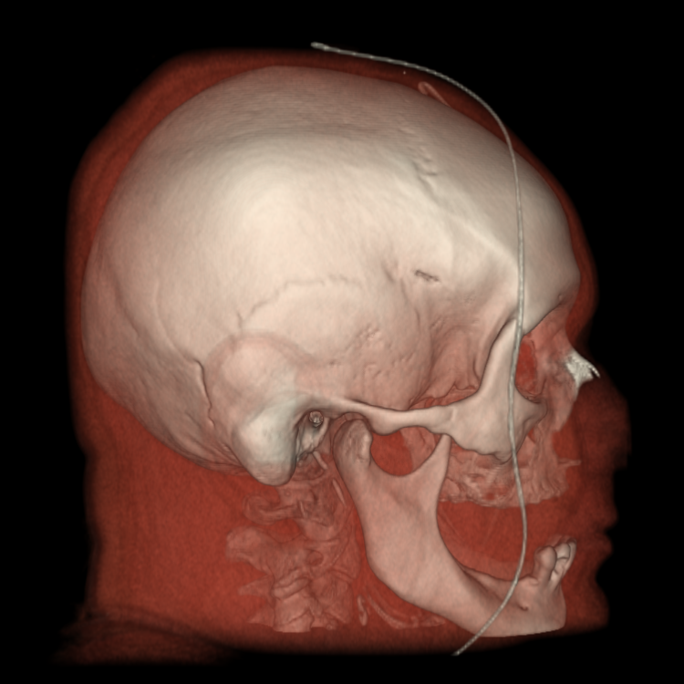 |
Part 3.1.4: Nose, eyes, and tissues The volume rendering captures a few interesting features that are not captured in the isosurfaceing. |
Part 3.1.5: Jaw, spinal column, and tissues Volume rendering provides a clear view of the bone structures whereas in the isosurfacing only a region of tissues are captured. There is also not a significant amount of details in the captured tissues. Also most of the jaw and spinal column are missing from isosurfacing. |
Part 3.1.6: Teeth and various tissues The volume rendering again captures a lot of details in the teeth and surrounding tissues that are not present in the isosurface rendering. The tissues in the volume rendering are more much precise and interesting. |
Part 3.2: Delta Wing Aircraft Simulation We found that while volume rendering can theoretically capture everything visualized using isosurfacing, isosurfacing captures some structures a lot more easier than volume rendering. Both approaches have advantages and diadvanages with respect to the lambda wing dataset. For instance, isosurfacing captures a bubble in the center using a very low isovalue while in volume rendering it is difficult to include and visualize this feature, especially if we are interested in capturing other features in parallel. Volume rendering using ray casting captures a significant amount of details within the vortices. Overall, the volume rendering using ray casting captures more vortices with more details in a simpler manner. However, for some minor structures that can be captured independently of any other features, such as the bubble, isosurfacing might be the better approach. We compare and contrast the two by applying the same classification color map to both ray casting volume rendering and isosurfacing and using consistent camera settings. |
Part 3.2.1: Top-view of vortices In the volume rendering using ray casting on the left, we are able to see vortices at the very tip of the wing by examining the structure closely. The vortices are subtle but extend all the way to the green structure in which they are no longer visualized. In the isosurfacing, we are only able to see what appear to be vortices by examining the cyan isosurface. The vortices/spirals are seen as minor holes in the cyan surface. They are definitely less distinct in the isosurfacing while using ray casting they are more detailed and 3D/spiral looking.  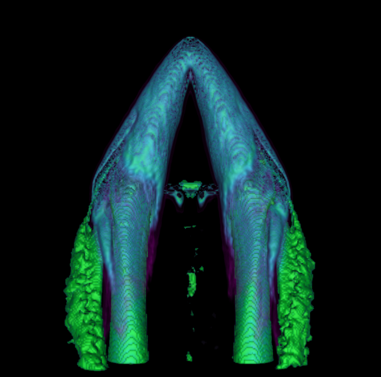 |
Part 3.2.2: Zoomed top-view of vortices On the left we are able to see what appears to be vortices/spirals when ray casting is applied. However with isosurfacing, we are unable to see any particular vortices. The reason is the spirals are captured using multiple isovalues therefore volume rendering with ray casting is more appropriate. 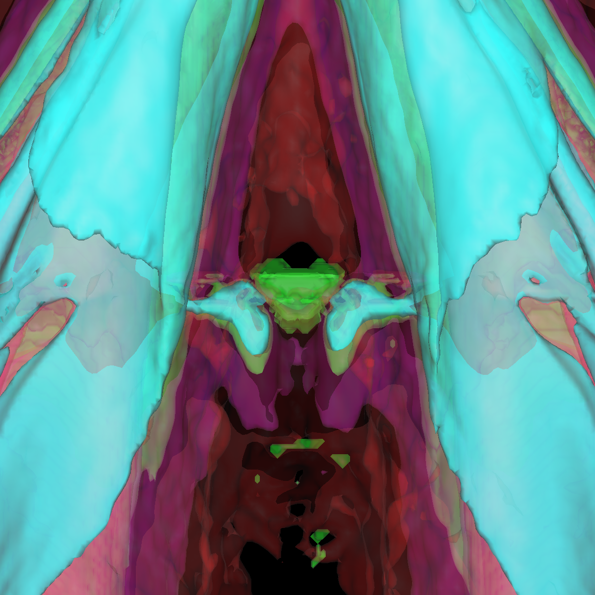 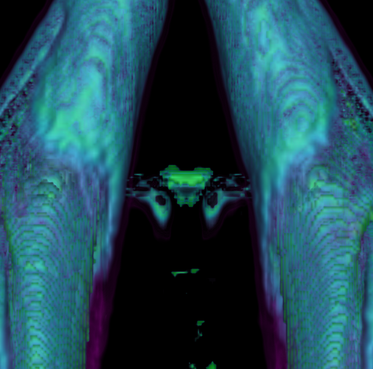 |
Part 3.2.3: Side-view of vortices In the ray casting volume rendering on the left, we see three vortices very clearly. First, we have the huge green vortices. Secondly, we also clearly see smaller spirals coming off of the green vortice as we move towards the front of the lambda2 wing. Another vortice is seen by looking directly above the green vortices. These vortices are clearly defined and very detailed as opposed to the isosurfacing rendering shown on the right. The isosurfacing rendering does not capture the smaller spirals/vortices coming from the larger green vortice. In the isosurfacing, transparency of the green vortice is an issue as if we make this structure more transparent, then we can no longer visualize the vertices from the top-view. However, besides this problem, the spirals are extremely difficult to capture using isosurfacing as mentioned previously.  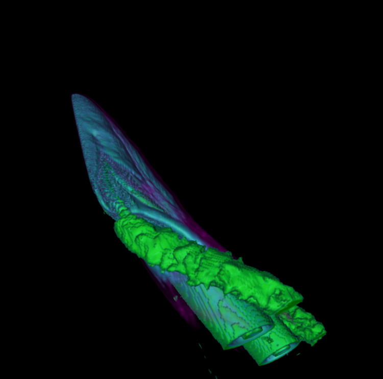 |
Part 3.2.4: Zoomed-in side-view of vortices The ray casting volume rendering on the right shows the spirals clearly, while the isosurfacing fails to capture this significant feature. 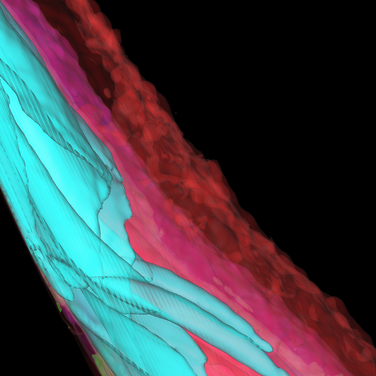 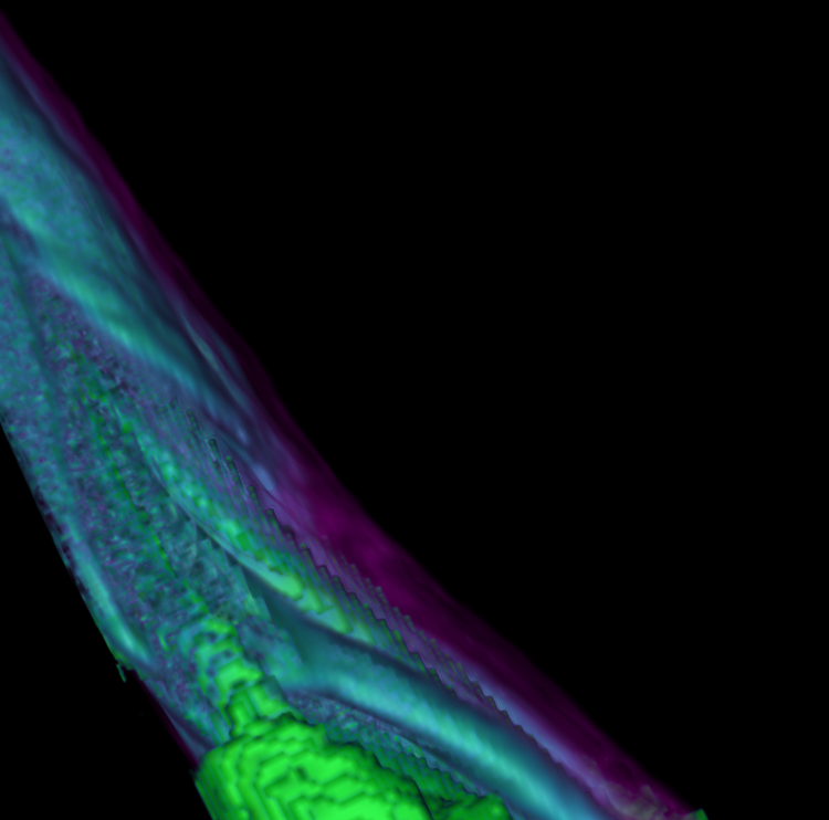 |
Part 3.2.5: Angled top-view The raying casting volume rendering on the left offers an angled view of the vortices where we can clearly see the vortices near the front and also the spirals farther down and the spirals forming the green structure. The vortices on the right are less visible and detailed and fails capturing certain spirals as described above. 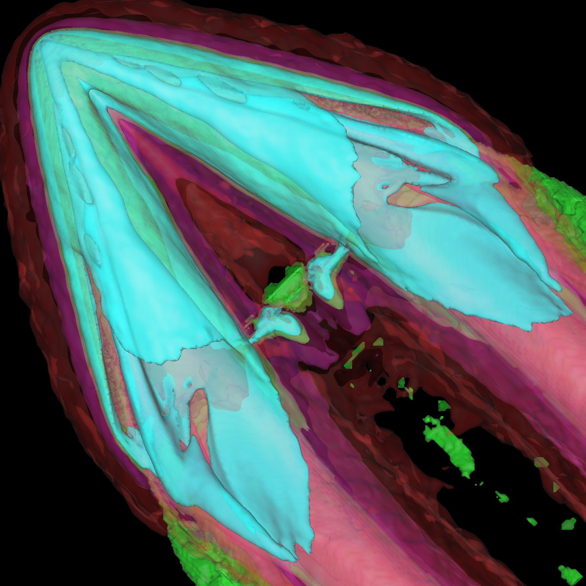 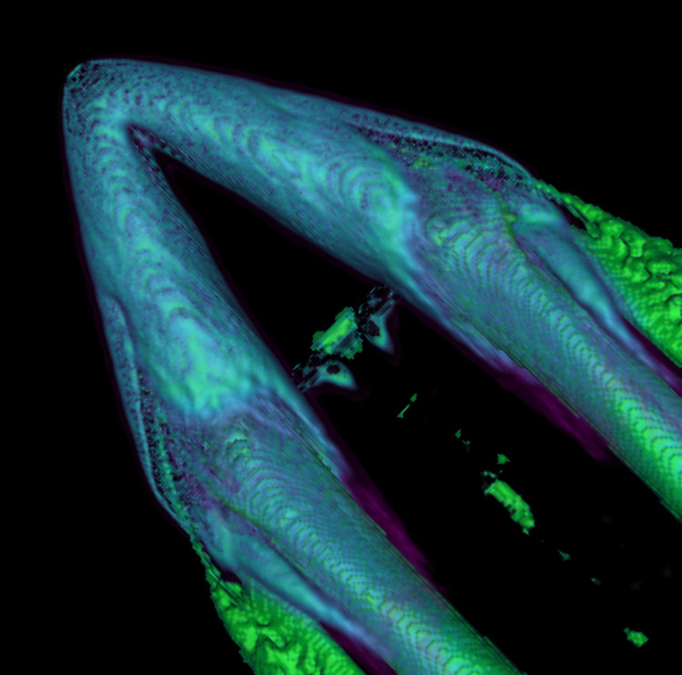 |
Part 3.2.6: View from the direction of the vortices The ray casting volume rendering on the left captures the large vortice, but fails to show any particular spiral. However, the cyan isosurface appears to capture the large spiral.  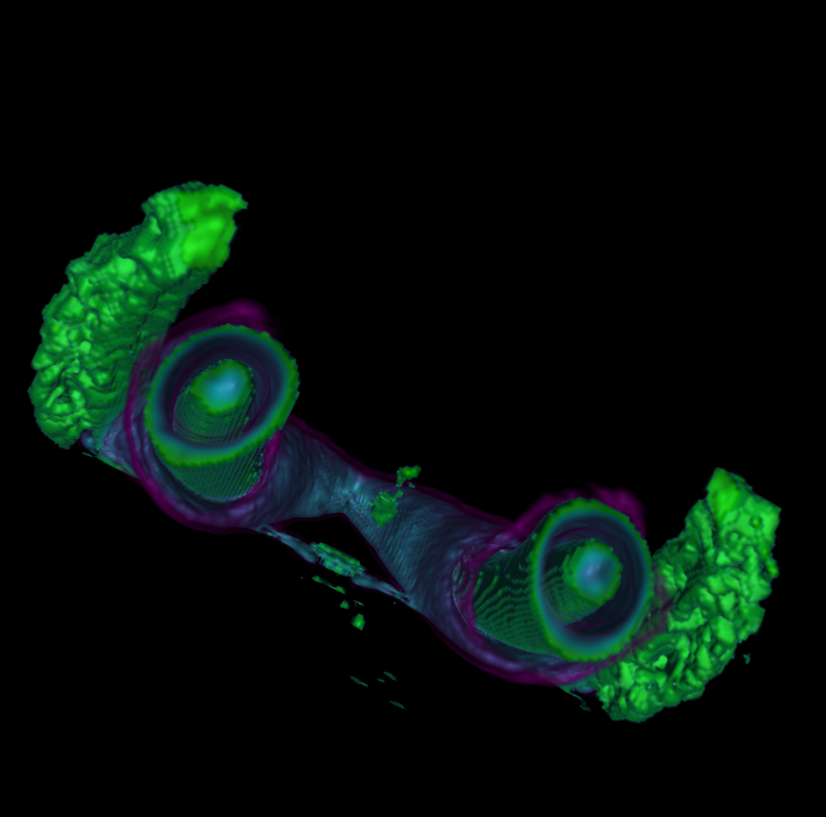 |
Part 4: Maximum Intensity Projection We apply Maximum Intensity Projection which in essence reduces the volume rendering integral to simply measuring the maximum scalar value along each ray. Once this is found, we designed two transfer functions; one for color and one for opacity. In particular, we define the following color transfer function [800-->Black, 1150-->Dark Gray, 1500-->Light Gray, 2000-->Lighter Gray, 3500-->White]. As for opacity, we define a piecewise function such that [800--> 0.0, 1150-->0.2, 1500-->0.3, 2000-->0.5, 3000-->1.0]. These functions immediately lead to a few interesting features. For instance, the teeth and what seems to be the jaw joint are explictly mapped to white.  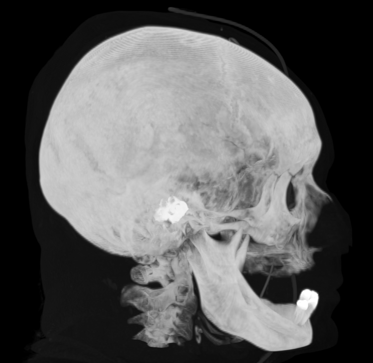 |
Part 4.1: Applying Clipping Planes to Volumes In this part, we apply clipping planes to the maximum intensity projection of the head CT dataset in order to extract interesting features. We show two screenshots below using the same visualization parameters, camera settings, and lighting as shown in the visualizations without applying a clipping plane. We decided to clip the volume in half; that is we slice the head in half by removing half the face with a vertical plane. As shown below, the clipping plane highlights other regions of interest which are unable to be captured in the original.  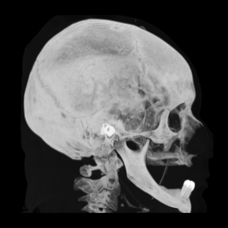 |
Part 4.2: Designing Multiple Transfer Functions for the Maximum Intensity Projections The Maximum Intensity Projections are traditionally one color (e.g., grayscale as seen in x-rays) and highlight regions with the highest density. However, we believe by using multiple colors to highlight the density differences and applying a suitable color map these regions could be further refined and made more visible for doctors and/or researchers. In particular, we are interested in more precisely defining regions of interest based on color (and opacities). In this light, we design many transfer functions for opacity and color and show what we believe to be the most significant visualization below. The other visualizations where we have explictly searched over in order to identify the most significant transer function are shown in section 4.4. 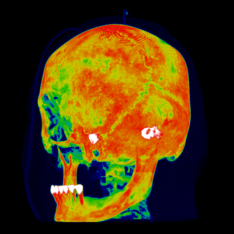 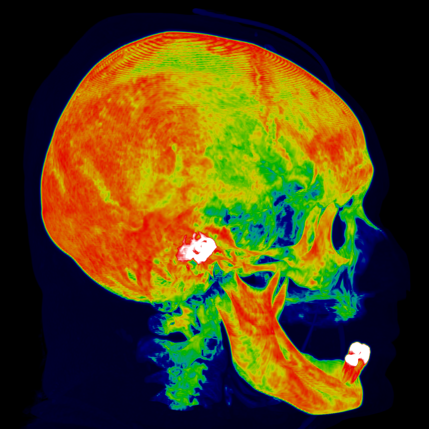 |
Part 4.3: Applying Clipping to the Selected Transfer Function We now apply the clipping plane described above to the most optimal transfer function. We again are able to find more details with respect to the face and densities. The clipping plane also enhances our ability to design the transfer functions as we expect similar densities would be found on the other side of the skull, therefore by reducing the skull in half allows us to more appropriately define opacities. The other half of the skull could be seen as redundant, depending on the task or goal of the visualization. 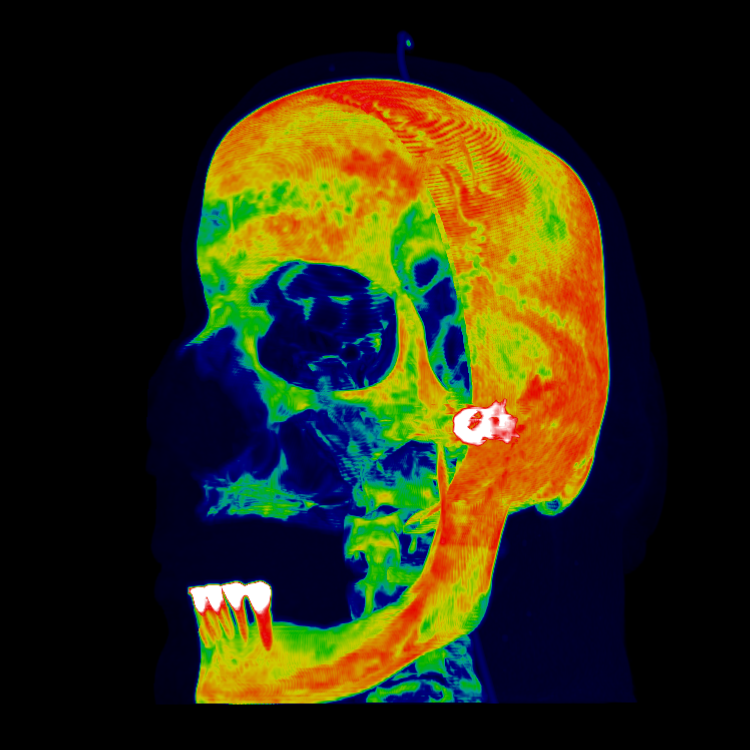  |
Part 4.4: Other Transfer Functions In this part, we show a few of the transfer functions for both color and opacity in which we searched over to find the most optimal.   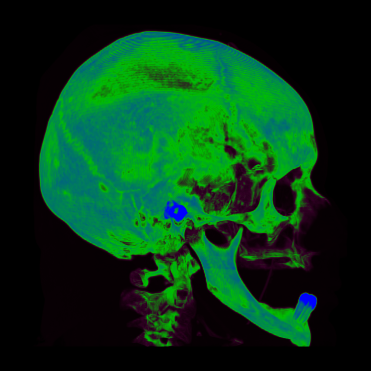  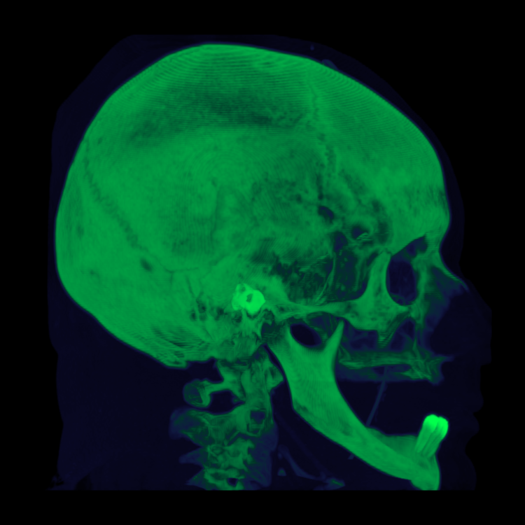 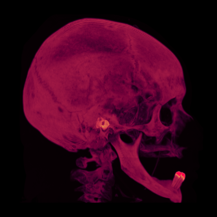  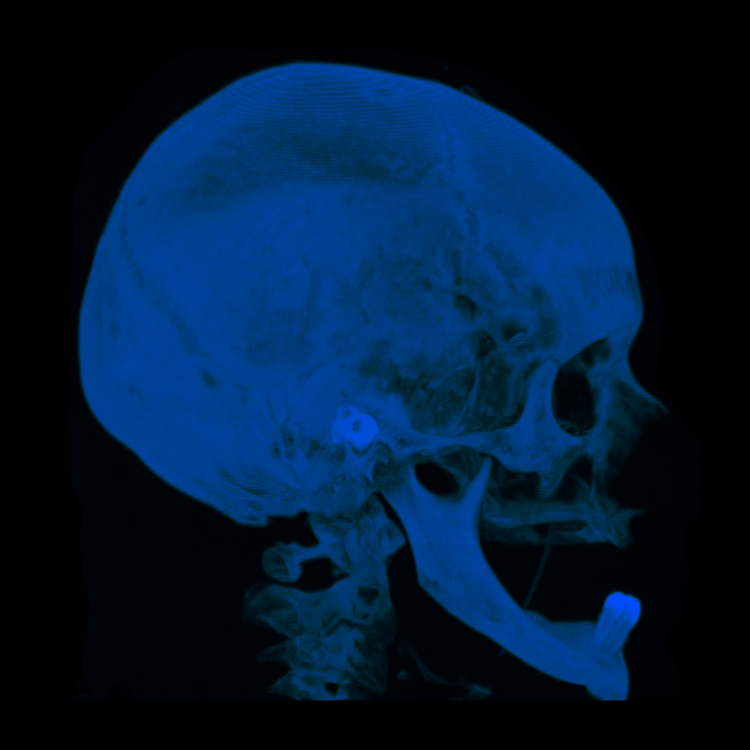  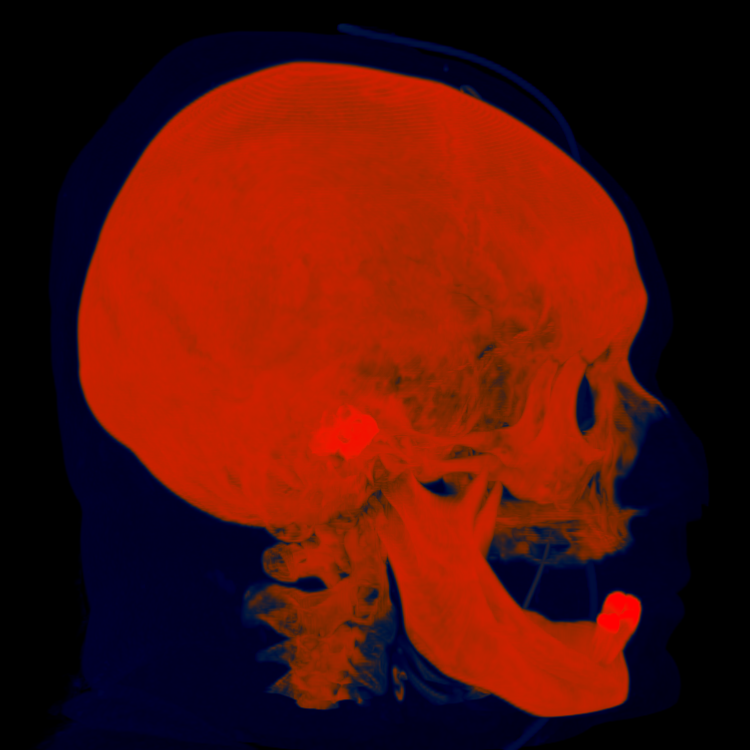 |
Part 5: Multidimensional Transfer Functions We design a multidimensional transfer function by using a combination of the scalar value and the gradient magnitude. More specifically, for each scalar value there exists an associated gradient magnitude value such that the values are combined by taking the product. In particular, the opacity is defined by the product of the scalar opacity transfer function and the gradient opacity transfer function. The significance of such an approach relies on the fact that just one value is sometimes not enough to characterize the boundaries of structures. However, more precise boundaries can be discovered and visualized by using a procedure that takes into consideration both the scalar value and the gradient magnitude. The disadvantage of such an approach is the significant increase of the space in which we need to search in order to identify more desirable boundaries. Perhaps this space could be pruned using some heuristics or insights making this approach more reasonable. Nevertheless, in datasets that significantly suffer by using only the scalar value, then the benefit of multidimensional transfer functions is immediately apparent. We designed the multi-dimensional transfer functions for the Head and Wing datasets by considering the homogeneous regions. In particular, the homogeneous regions with a constant rate of change are made drastically more transparent or even eliminated. This allows for other interesting features to be captured. In particular, the multi-dimensional transfer function designed for the head drastically improves our ability to detect the brain/white matter when applying a clipping plane (shown in section 5.1.1). For the wing dataset, we designed many different multi-dimensional transfer functions. The most significant multi-dimensional transfer function captures the inside of the large green vortices among other features. |
Part 5.1: Designing Multidimensional Transfer Functions for the Head CT Dataset We used the color transfer function defined previously. For these renderings the scalar opacity transfer function is defined as [0->0.0, 800->0.5, 1050->0.1, 1600->1.00] and the gradient opacity transfer function is defined as [0->0.0, 90->0.5, 100->1.0]. We selected the gradient opacity transfer function with the motivation to decrease the opacity in the volume regions where the rate of change is not significantly different (e.g., tissues). However, we designed the opacity function such that these flat regions would still be maintained at the boundaries. A boundary can be seen as any significantly different rate of change between regions and therefore by this definition we are able to capture different tissue types and features of the tissues. The utility of the multidimensional transfer function is shown by comparing the visualization using the one dimensional transfer function with the visualization using the multidimensional transfer function. The improvement is significant. The significance of using a multi-dimensional transfer function is further shown in the next sections where we use clipping planes and other methods to capture interesting features.  |
Part 5.1.1: Applying Clipping Planes to Multidimensional Transfer Functions The significance is shown further in our feable attempt at visualizing the white matter and other more reasonable structures. We chose to clip the volume in half; that is we slice the head in half by removing half the face with a vertical plane. As shown below, the clipping plane highlights other regions of interest which are unable to be captured in the original. The product of the scalar opacity transfer function and the gradient magnitude transfer functions defines the regions for which the directional magnitude does not significantly vary. In particular, the multidimensional transfer function assigns the tissue to be more transparent allowing for us to clearly see other interesting features. The tissues are difficult to capture using isosurfaces, but with volumes they are quite easy and they impact the ability to capture other significant features. Using only the scalar value to map the opacity does not allow us to capture these interesting features as we already know that there does not exist any one particular value that captures the tissue. Therefore, we designed the multi-dimensional transfer function around this idea; that is we are not interested in the homogeneous regions between different tissue types. More specifically, we eliminate these homogeneous regions by assigning them to be transparent, while making the boundaries between the tissue types more opaque. In this light, the multidimensional transfer function could be considered a way to reduce the dimensionality and/or the significance of structures that dominate the feature space. The multidimensional transfer function reduces the dimensionality by also considering the rate of change as a factor in determining the opacity. In the two examples below, we demonstrate the signifiance of the multidimensional transfer function based on both the scalar value and gradient magnitude and compare it to using only the scalar value. 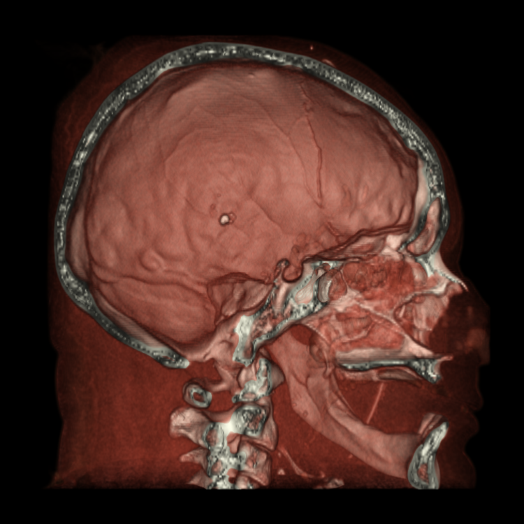 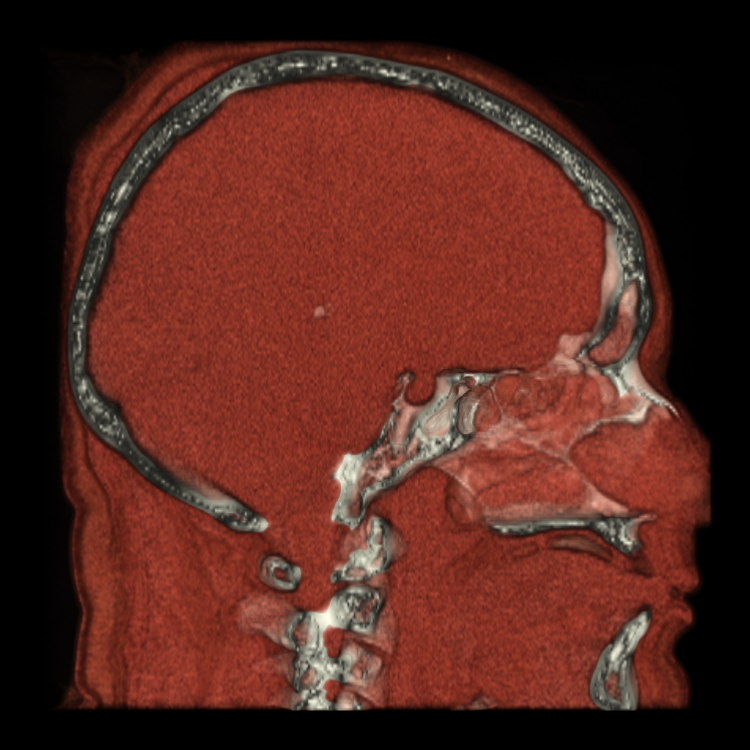 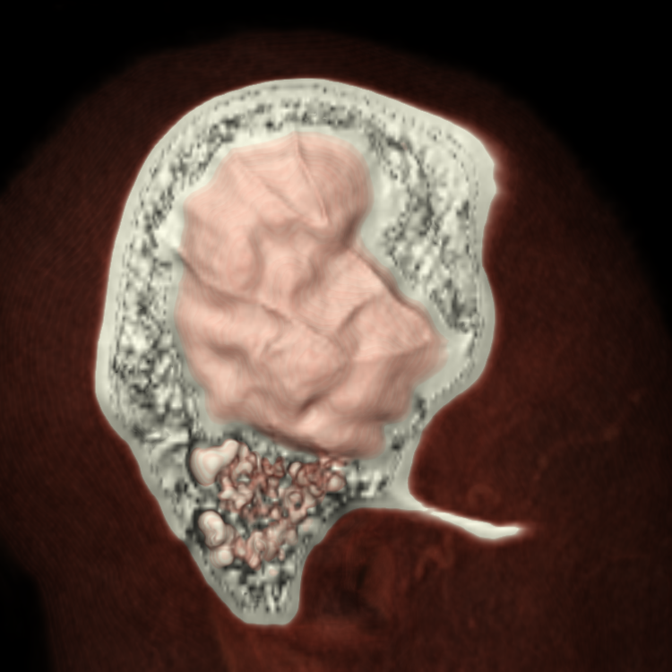  |
Part 5.1.2: Other Interesting Features from Multidimensional Transfer Functions We show a few examples of other interesting features in which we extracted by applying multidimensional transfer functions. 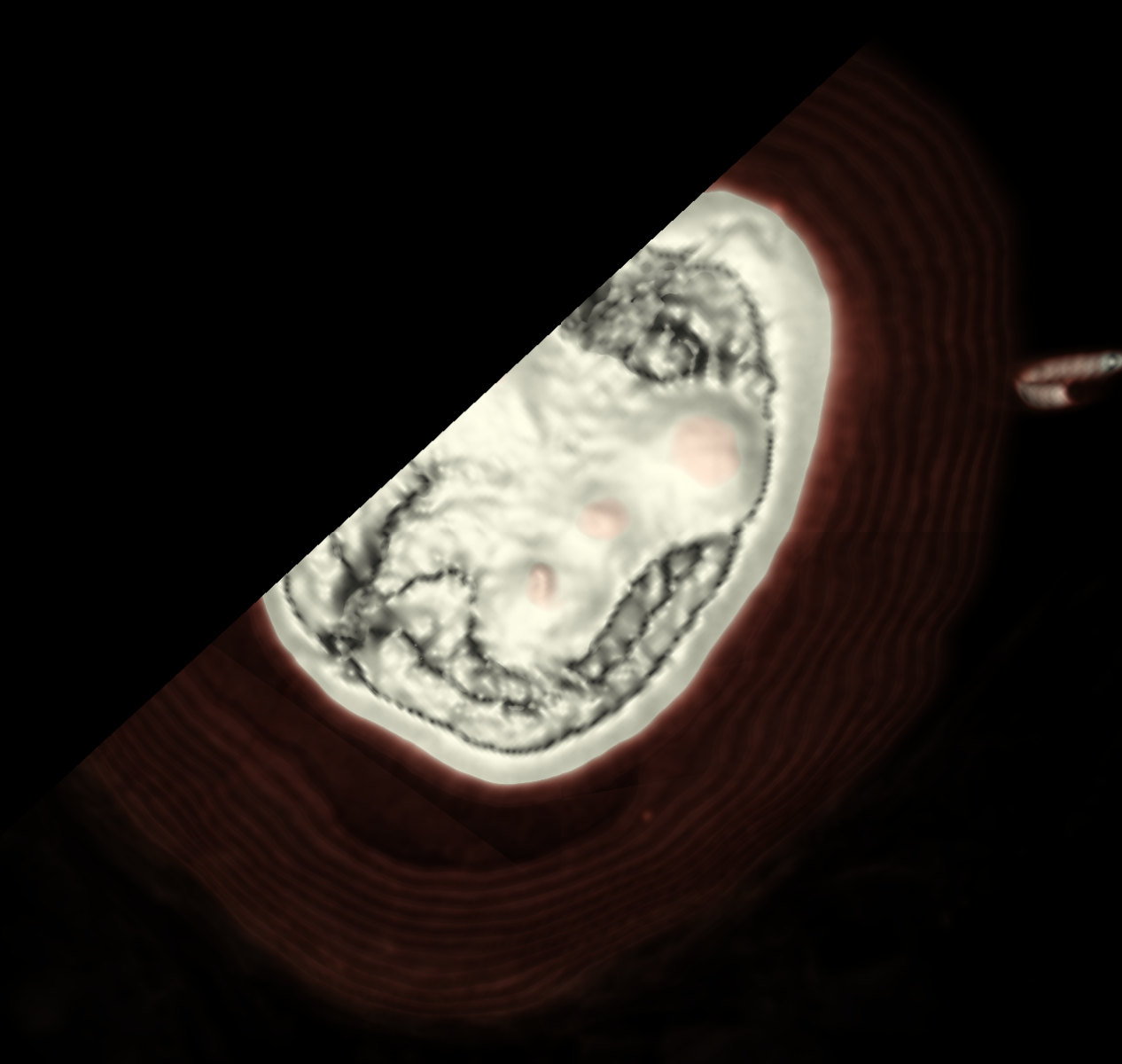   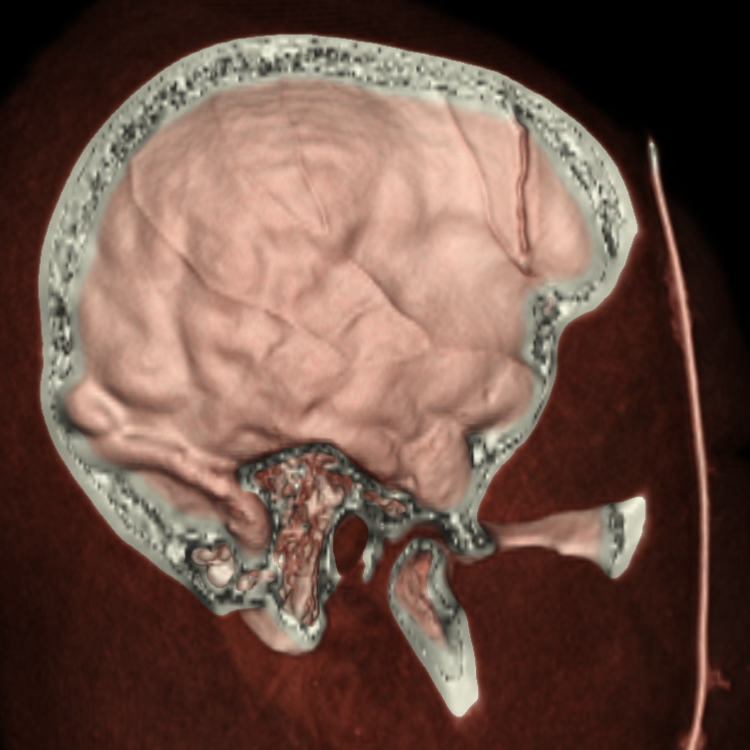 |
Part 5.1.3: Maximum Intensity Projection using Multidimensional Transfer Functions In this rendering we attempt a maximum intensity projection using the previously defined multidimensional transfer function. We compare the results to two baselines. The first baseline is a maximum intensity projection using only the gradient magnitude transfer function. The second baseline is the maximum intensity projection paired with the scalar based transfer function. The first screenshot on the left is the maximum intensity projection using a multidimensional transfer function, the middle is the scalar value and the rightmost screenshot is the gradient magnitude. The multidimensional and scalar value renderings are nearly identical. This is expected since the maximum intensity projection only considers the maximum values thus we do not have this issue of tissues or other flat surfaces. However, using only the gradient to map the opacity provides a much more different and interesting rendering as shown in the rightmost picture. 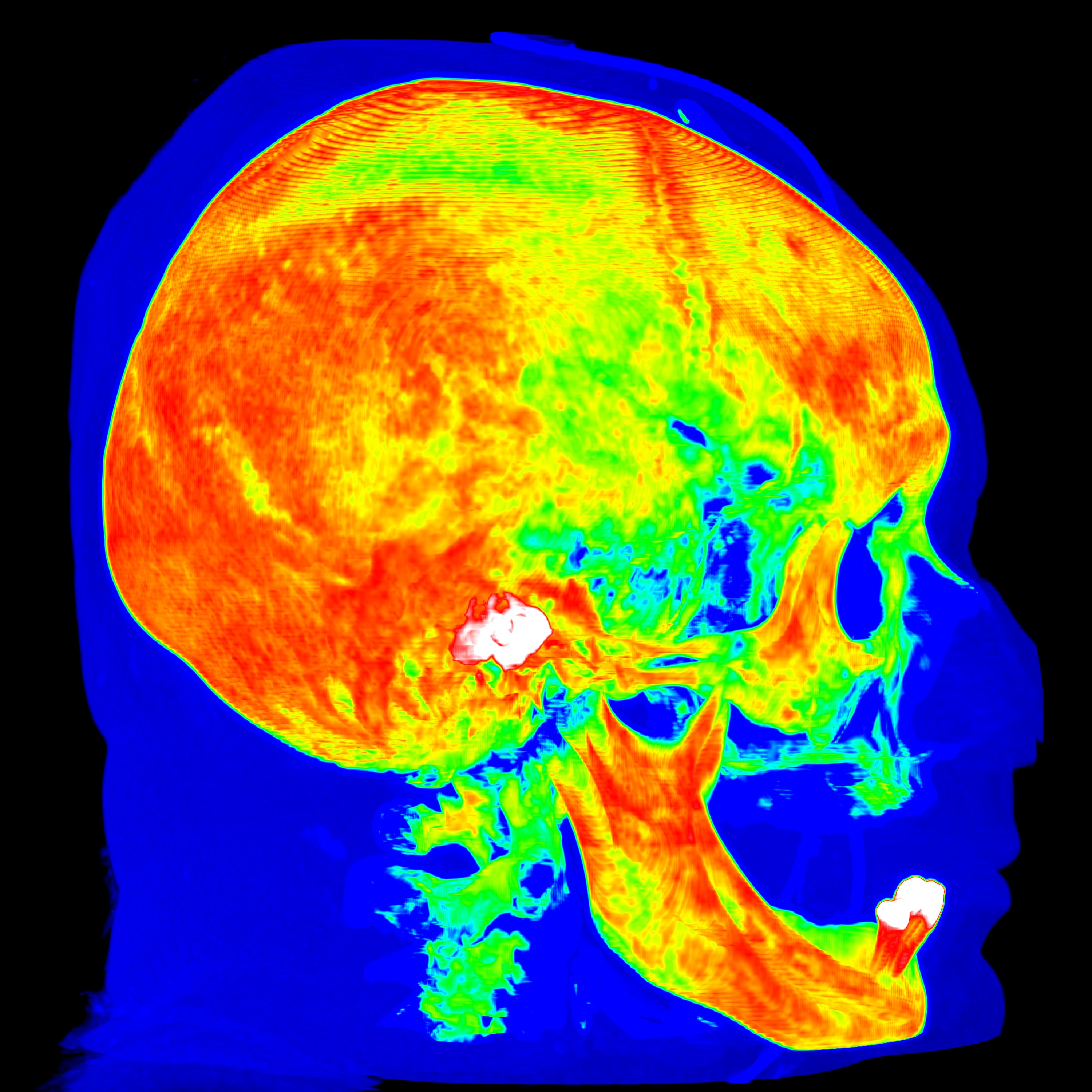 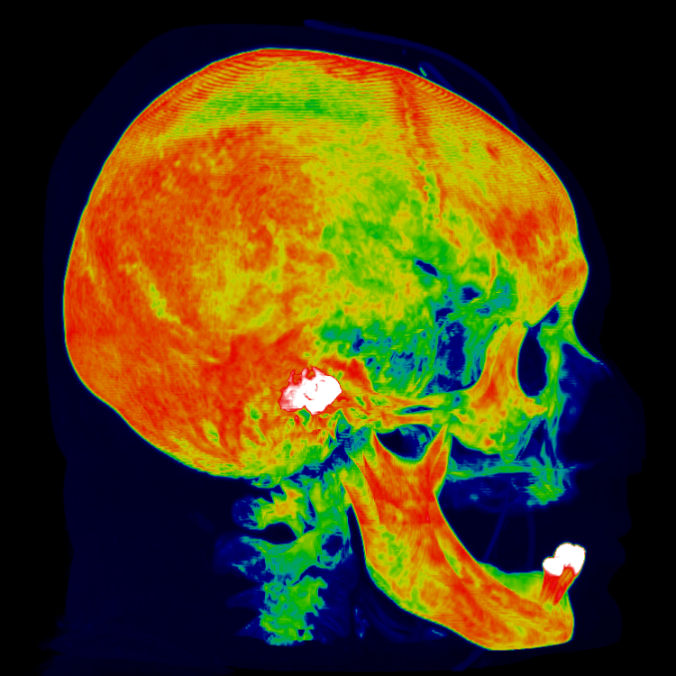  |
Part 5.1.4: Trilinear vs. Nearest Neighbor Interpolation We compare using trilinear interpolation and nearest neighbor interpolation while applying the multidimensional transfer functions described previously. The trilinear interpolation is definitely more precise allowing for sharper renderings. 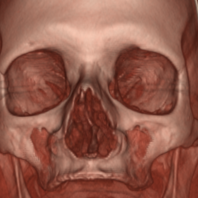 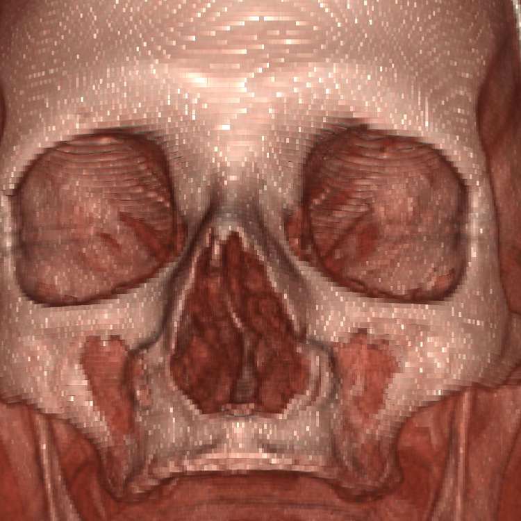 |
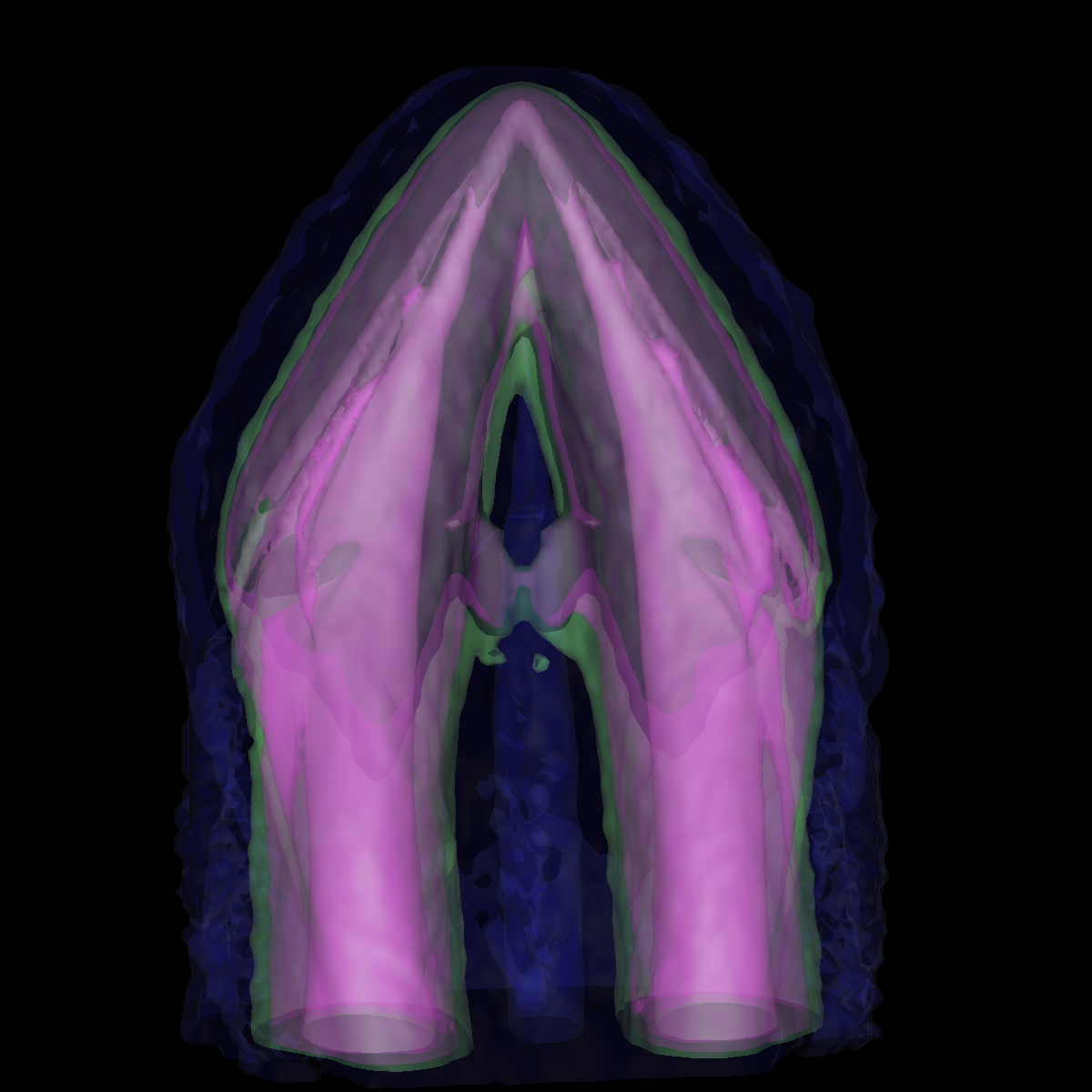
Part 5.2: Designing Multidimensional Transfer Functions for the Wing We designed various multi-dimensional transfer functions for the Wing Dataset. First, we defined the following classification color map {35000->pink, 50000->cyan, 60000->green} for the different features/vortices. As for the multi-dimensional transfer function, we defined the scalar opacity transfer function as {35000->0.0, 50000->0.1, 60000->0.50} and the gradient magnitude transfer function as {140->0.0, 150->1.0, 180->0.0, 250->0.0, 260->1.0, 300->0.0}. We designed the gradient transfer function by analyzing the gradient values and identifying the regions to which each correspond. As regions are most likely changing at different rates, but the gradient at some scalar associated with a vortice might be equal to some other regions vortices. The multi-dimensional transfer function improves the visualization as shown below. In particular, the multi-dimensional transfer function captures the details of the green structure more accurately. We are also able to see the inside of the green structures and in particular the significant contours that seemingly form spirals. Furthermore, we are able to visualize vortices/spirals beside the green structure whereas with the one-dimensional scalar based transfer function we fail to capture the vortices inside the larger one and miss a significant amount of detail. The multi-dimensional transfer functions are definitely more useful, but designing them is an even more difficult problem as it adds another level of complexity. The potential benefit will depend on the particular dataset. The multi-dimensional transfer functions could possibly be designed semi-automatically by using heuristics from the scalar values and the associated knowledge of the structures. The ultimate goal of a multi-dimensional transfer function for the wing dataset would be a function such that the noise other than the distinct spirals/vortices are assigned to be transparent while the boundaries between spirals/vortice types are captured. This particular multi-dimensional transfer function is extremely difficult to identify using the untransformed lambda2 dataset. 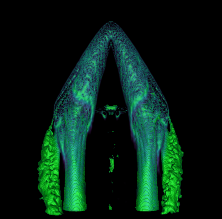  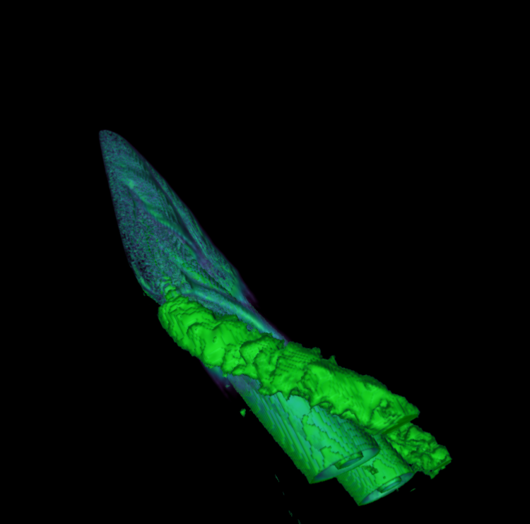 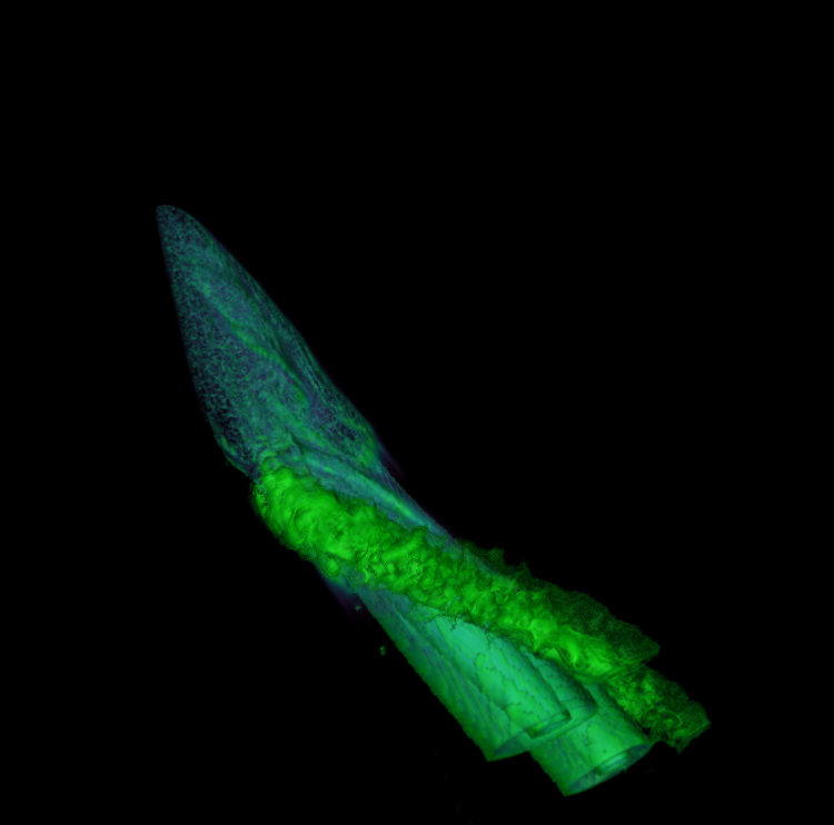   |