Isosurfaces and Clipping Planes to Visualize Anatomical Structures
 We created a self-contained GUI for this project since most of the code between parts did not change significantly. The GUI has the advantage of exploring each of the datasets very easily once all the visualizations were coded. We have attempted to make the GUI as easy as possible to use for grading. However, it could become confusing, so we have included details to understand the motivation of the GUI so that different project components can be easily assessed and the correctness verified. We have included a screenshot of the GUI above. For instance, if we wanted to visualize the head using the large dataset and also wanted to include transparency and a clipping plane then we could easily do so by simply pressing the buttons corresponding to each feature explictly written on the GUI. |
Part 1: Extract and Visualize Anatomical Structures using Isosurfaces In this part, we explain the problems associated with capturing each of the anatomical structures using a specific isovalue and give intuition on the reason for this inconsistencies. We chose a realistic color map for both the head and feet where once we identify the isovalues that give the best results we also use those values as a mapping to realistic colors for bones (white), tissue, skin, and white matter. Interpolation is used to assign similar colors to isovalues that are close to the finite set of isovalues we explictly assigned to colors. |
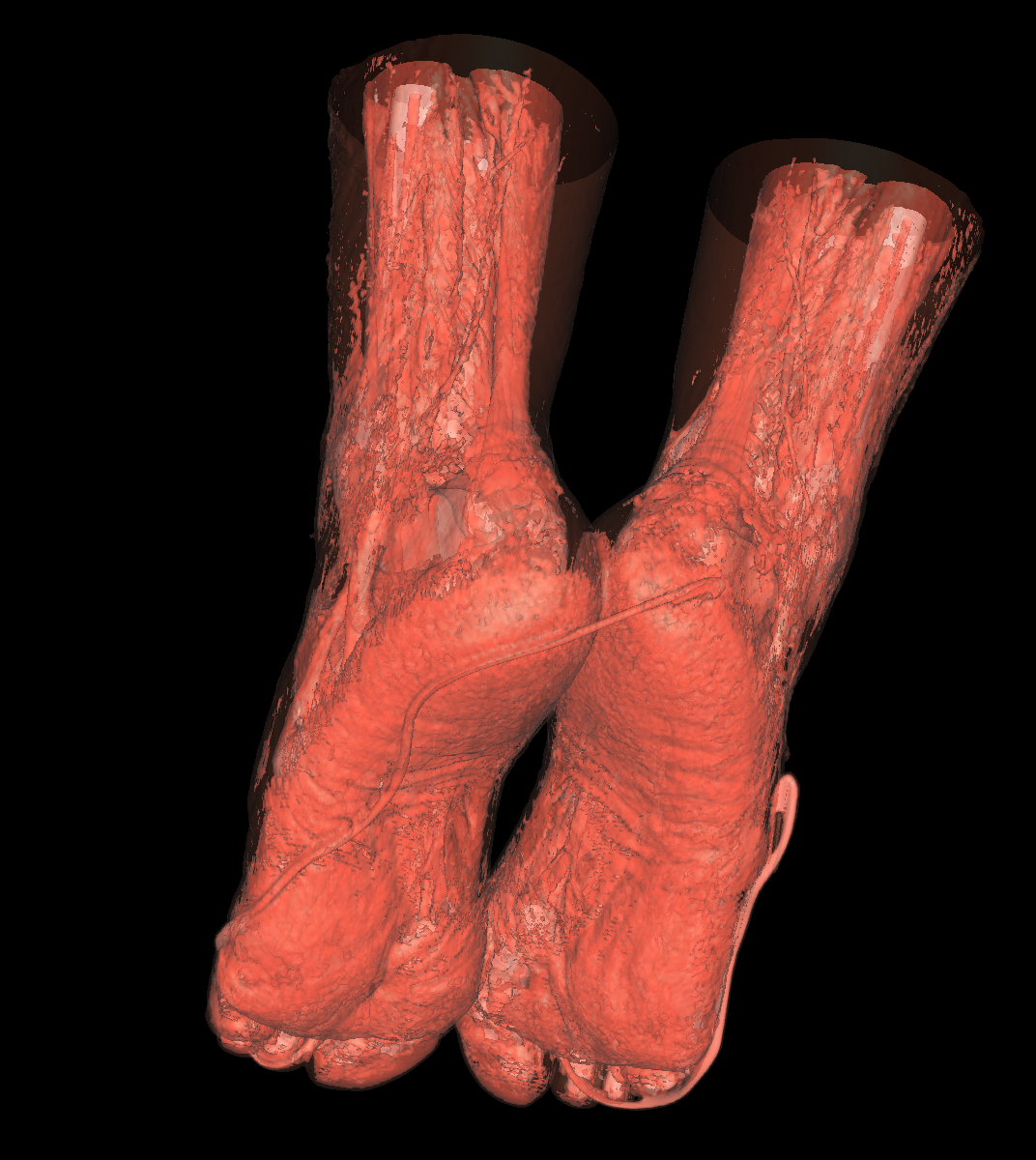
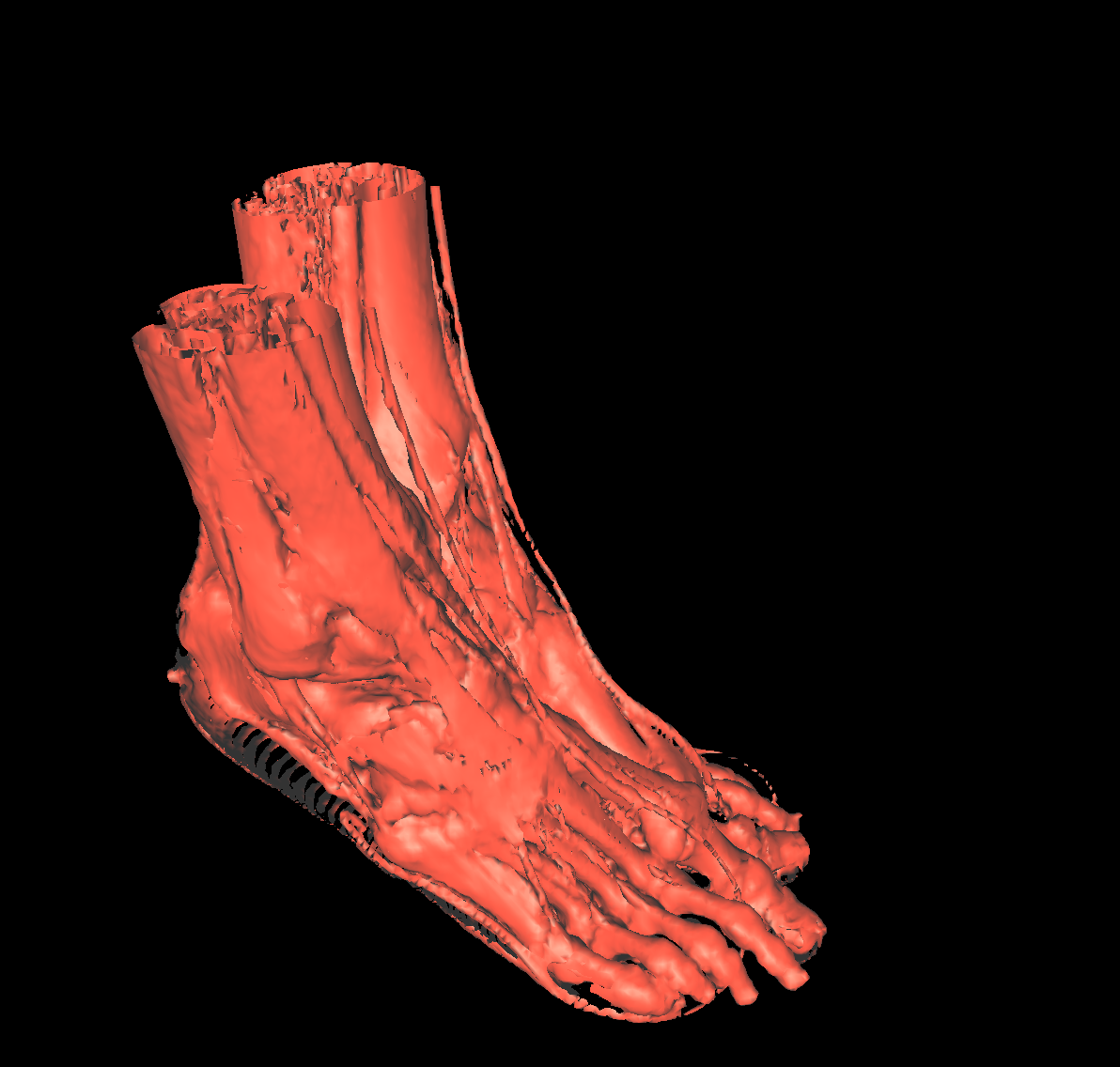
Skin: The skin is relatively easy to capture using a particular isovalue (i.e., the range of isovalue is quite large). We chose an isovalue of 700 for both the feet and head. The head needed a higher isovalue to capture part of the nose which was not captured by 500 and various other isovalues. The skin is probably the least interesting anatomical structures. We show two screenshots of the visualized skin for both the head and feet using the classification color mapped described previously. 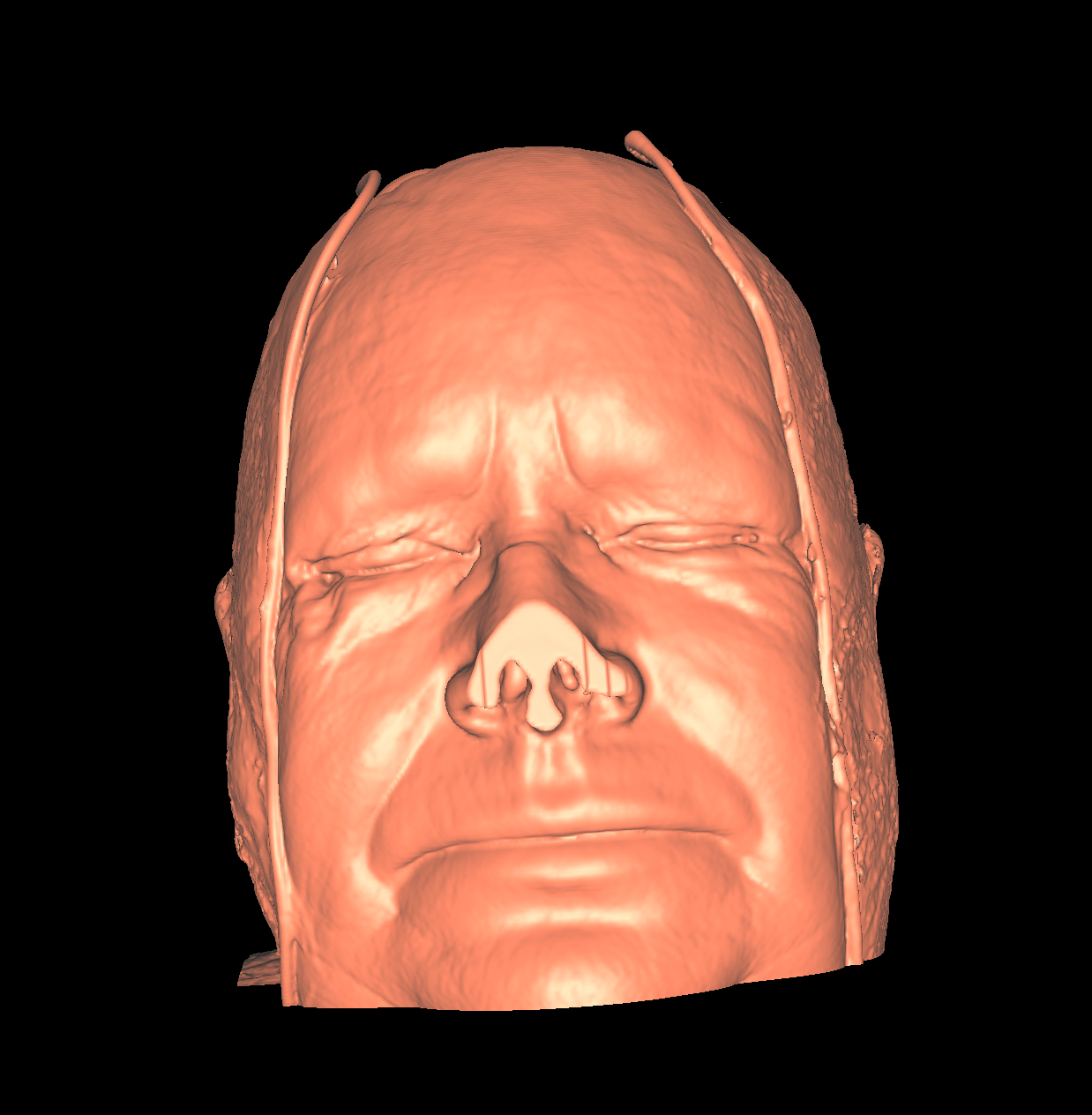 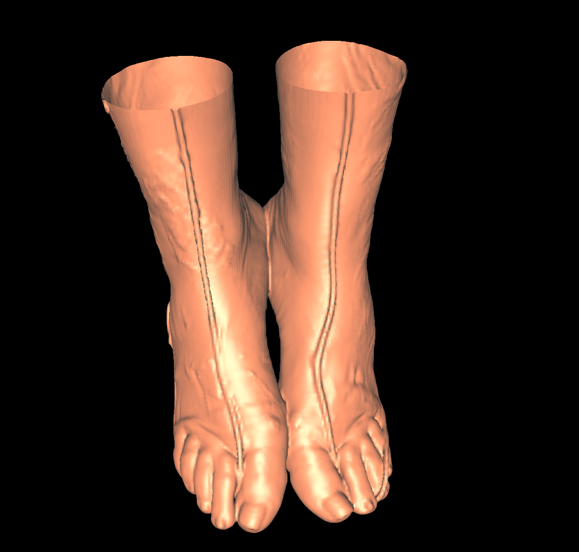 |
Soft Tissue/Muscles: The tissue is probably one of the most interesting isosurfaces, but remains very difficult to visualize using only one specific isovalue. For instance, we chose an isovalue of 1050 for the feet and head in order to partially capture the muscle and tissues. The head tissues are even more difficult to visualize. However, by increasing the isovalue slightly, we immediately start seeing bones while decreasing it slightly we immediately start seeing skin. There is not one single isovalue in which the soft tissue/muscles are captured. This causes holes in our surface. In essence, the isosurface fails if the tissue/muscle or any other anatomical structure oscilates. One potential solution is to smooth/convolve the surface by considering other values around a specific isovalue. The tissues would be better visualized using transparency with multiple isosurfaces to bring out the interesting features. Another option would be to visualize the CT scans as volumes. The intuiton is that volume rendering is roughly equivalent to rendering an infinite number of isosurfaces nested within one another. We show a few screenshots of the visualized tissue for both the head and feet using the classification color map described previously. 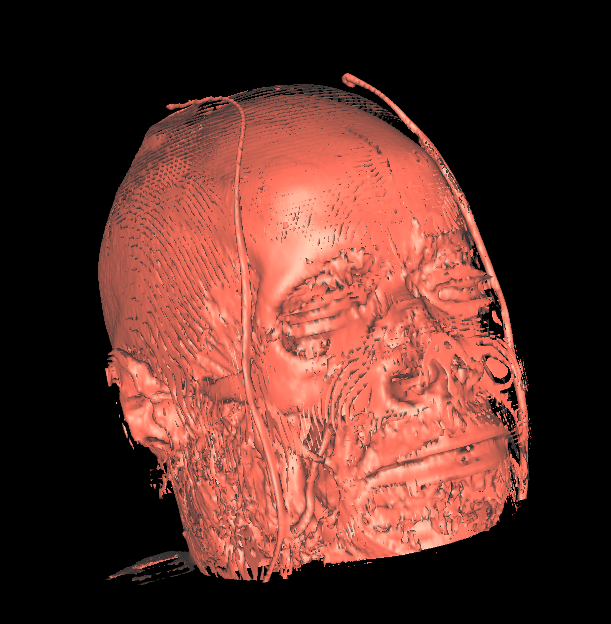  |
Bone: The bone is relatively easy to visualize as there are a wide range of isovalues that capture the bone structures in both the head and feet. Besides the challenging problem of visualizing soft tissue with a particular isovalue, we found that the bone structure contained interesting features while varying the isovalues. We show a few screenshots of the interesting features from the visualized bone for both the head and feet using the classification color map described previously. For the bone, we chose an isovalue of 1150 for both head and feet.  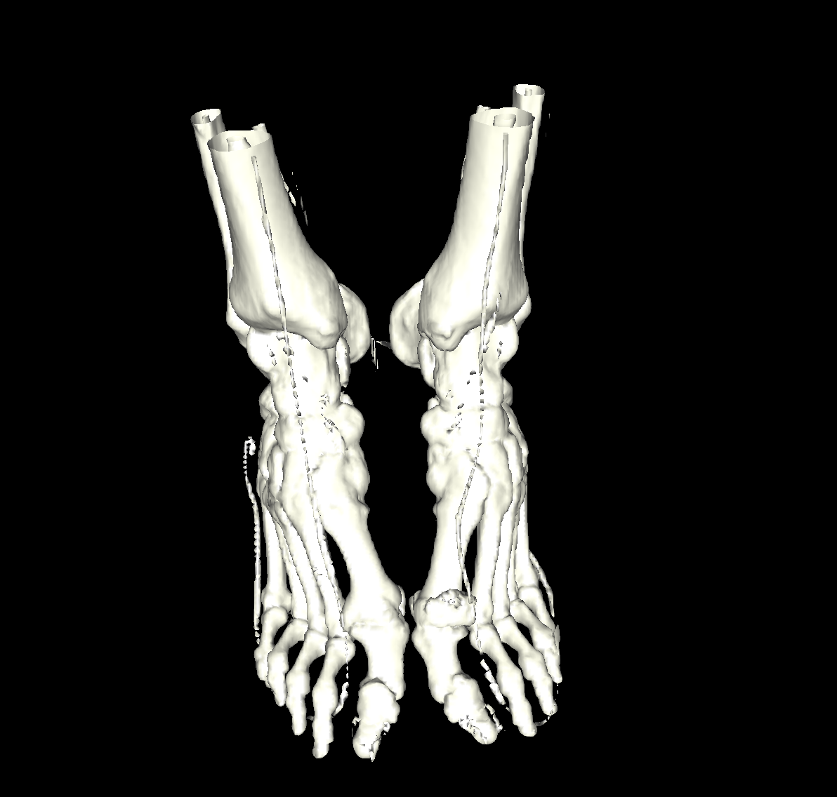  |
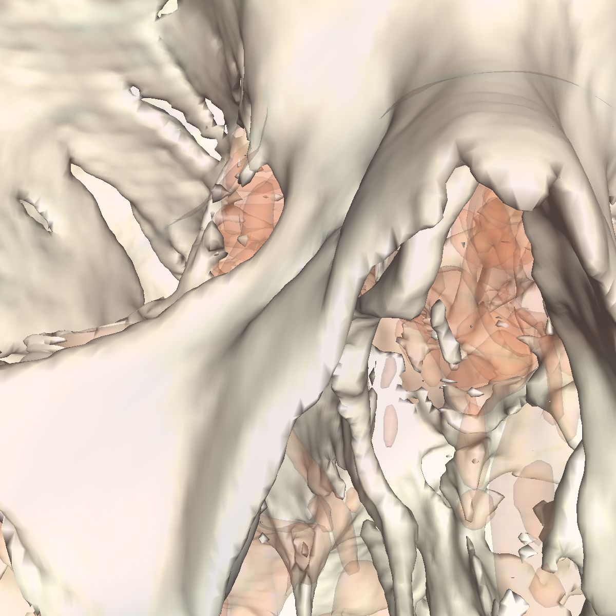
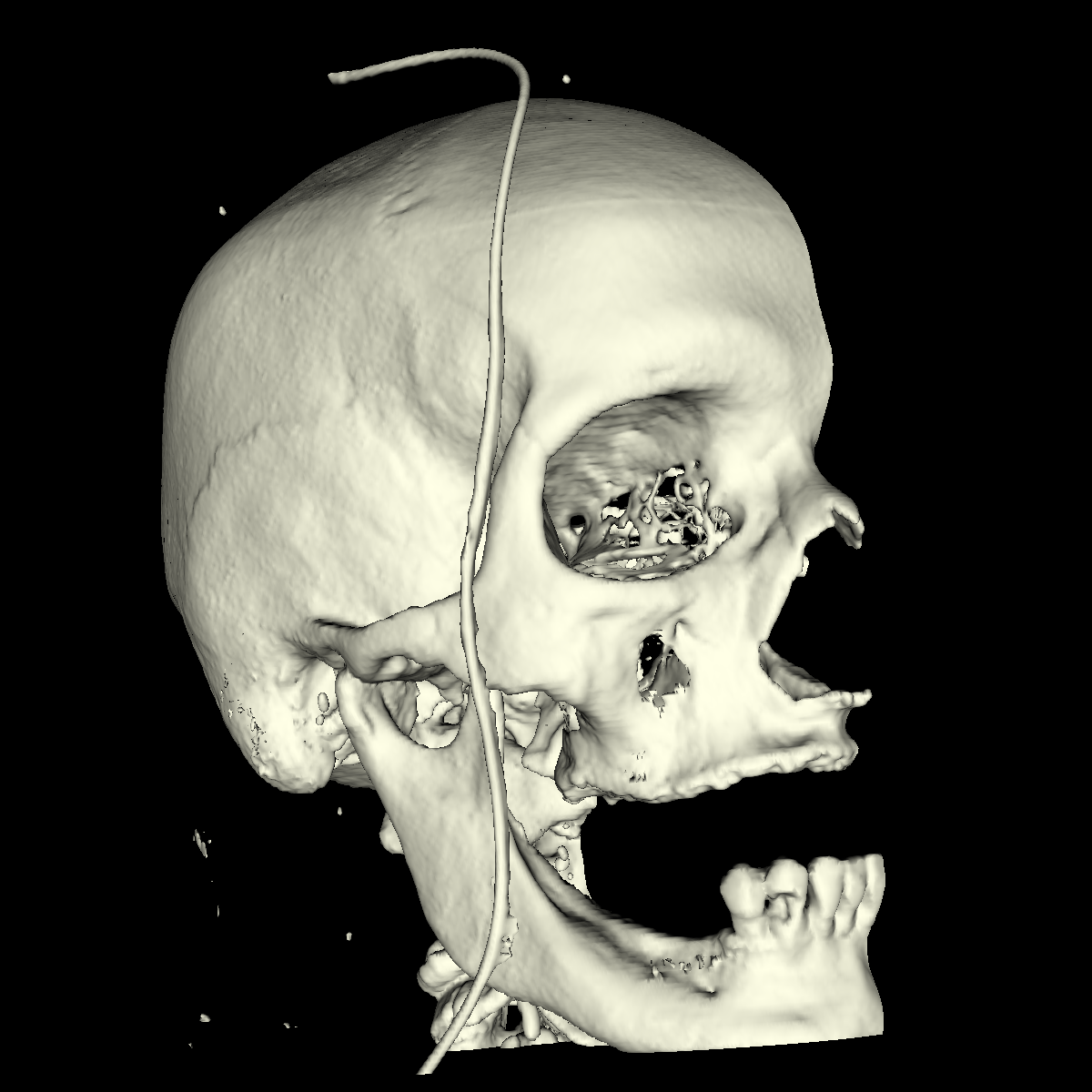
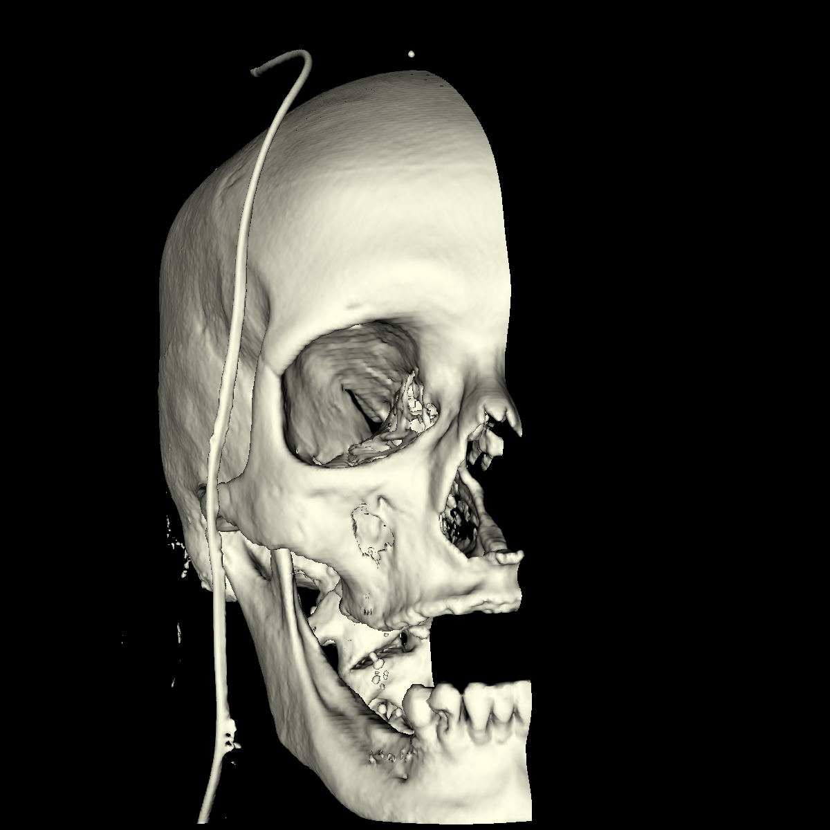
White Matter (Brain): The white matter is very difficult to visualize using one specific isovalue since the white matter from the brain is covered by the skull and to remove the skull from the visualization we already need to choose a very higher isovalue, so once we find this value, we also lose most of the white matter. If the skull was not there, then capturing the white matter would be significantly easier. For this part, transparency is definitely required. Finally, we show screenshots of the pieces of white matter in which we were able to visualize. A few artifacts of the white matter can be seen by looking through the eye in the screenshot on the left (i.e., we chose an isovalue of 1550). In the other screenshot, we also see a few artifacts of white matter by looking at a slightly different angle with an increased isovalue of 1900. It seems this problem of visualizing the white matter stems from the way the data was obtained. In that the values seem to correspond to density (i.e., things with lower densities corresponds to lower isovalues while structures with higher densities correspond to significantly higher isovalues. This could be an issue since the skull has a significantly higher density than the white matter underneath the skull.  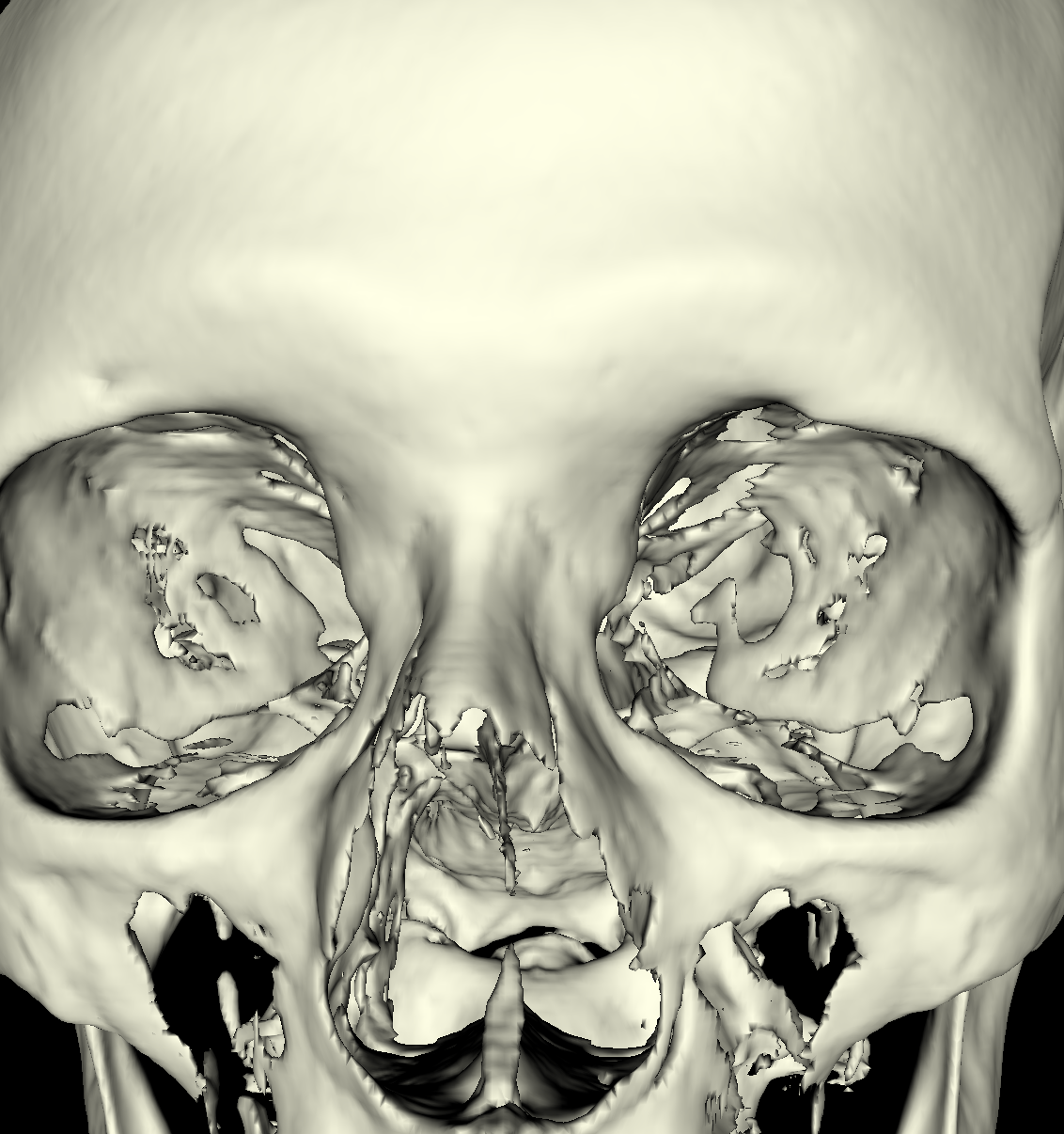 |
Part 2: Isosurfacing the Gradient Magnitude of the Volumes We now turn our attention to the magnitude of the gradient for the volumes. We applied the probeFilter to display the gradient magnitude as suggested. Doing this, we found the range to be completly different causing us to create colorTransfer functions for both the head and feet magnitude datasets. We used the same color map (i.e., classification color map) for visualizing the gradient magnitude datasets. The colorTransfer function was designed by studying the evolution of isovalues and choosing the optimal values that best highlight the anatomical structures (Head: Skin=20000, Tissue=40000, Bone=60000; Feet: Skin=20000, Tissue=40000, Bone=50000). One noticable difference is that the magnitude values are extremely large compared to the original dataset. The surface also appears to be smoother/softer using the magnitude values. However, the surface is also less continuous as there are frequent holes as the magnitude values capture the surface with approximations, but these values are not optimal/required for all isosurfaces and thus causes holes in the more precise isosurfaces. Indeed, we saw this idea in the previous visualization where it was extremely difficult to appropriately visualize the tissues due to the values oscilating. We mentioned that one idea would be to apply smoothing to this surface so that approximations of the values are assigned as a means to capture some of the oscilating structure. However, as seen in this visualization, the trade-off of smoothing a surface is that very precise surfaces that do not oscilate now contain holes in various places. Nevertheless, it is again very difficult to capture the tissue and the white matter. In the screenshot below where we attempt to capture the tissue, you can see that the mouth is somewhat cut out as well as other regions. The gradient magnitude tells us more on how the data was generated or measured such as densities which is also seen clearly from the magnitude datasets. The regions with a higher density are more visible whereas the original datasets are more continuous as shown by comparing the screenshots. 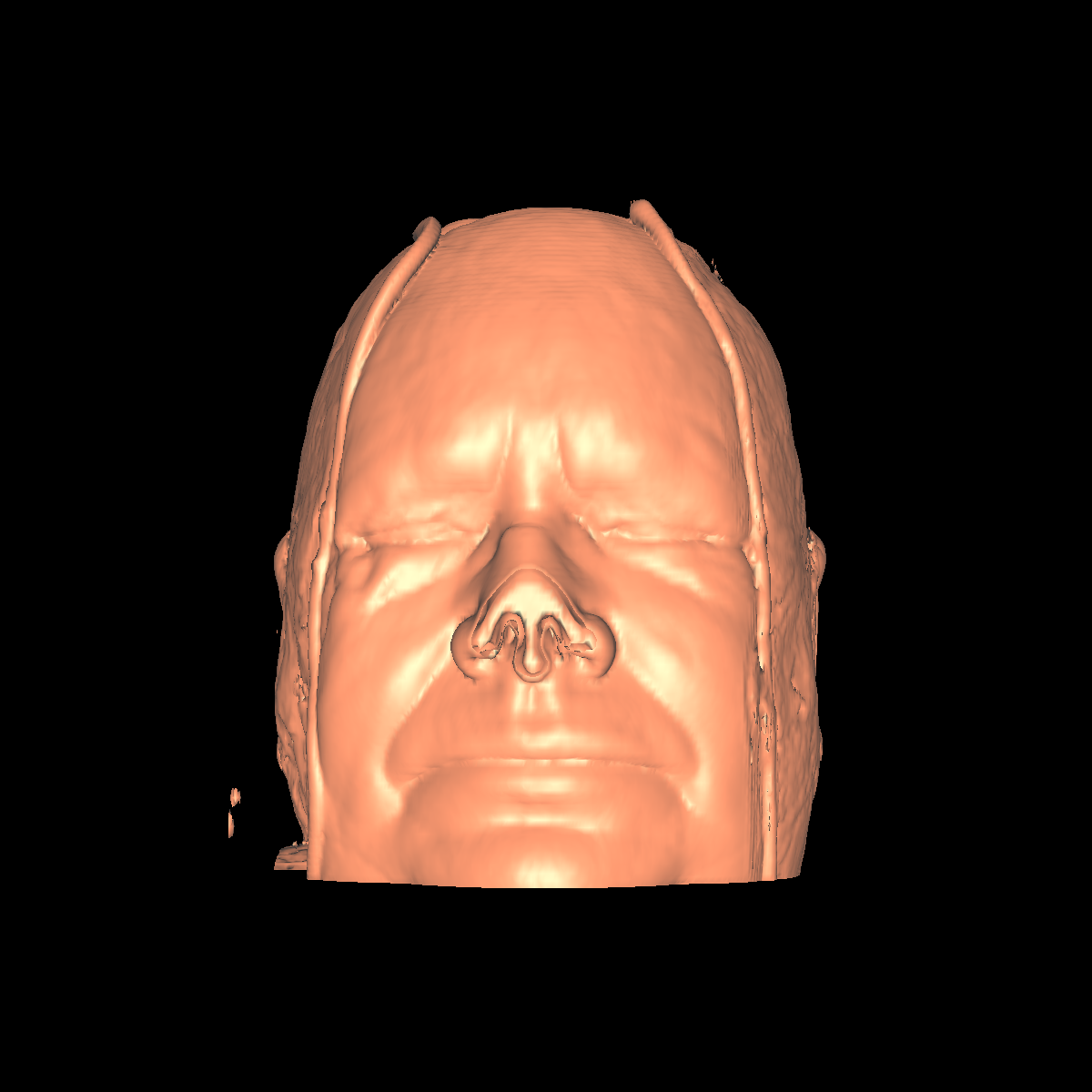 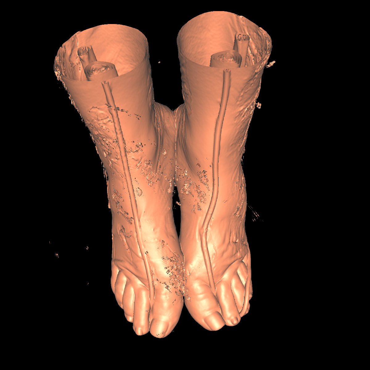 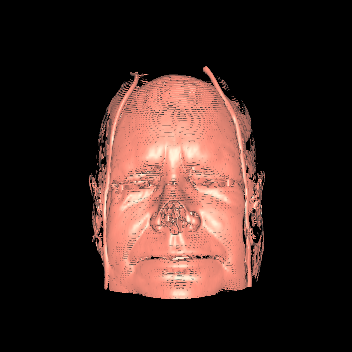 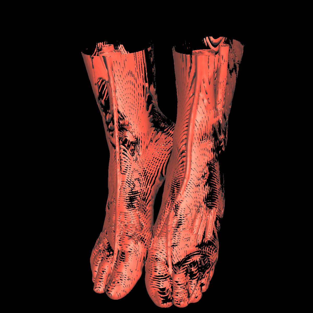  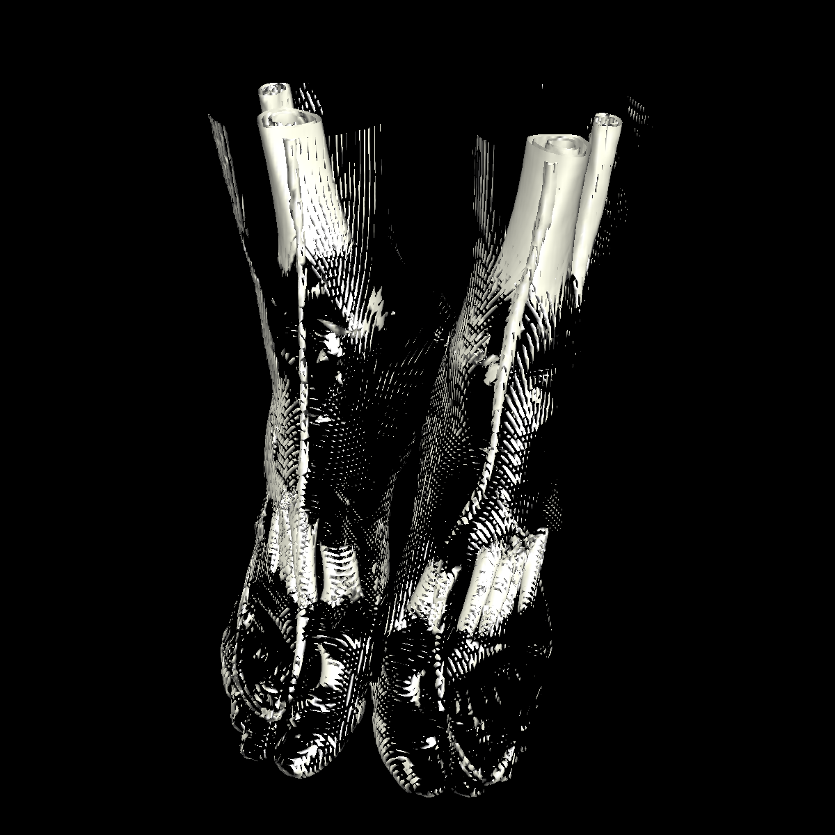 |
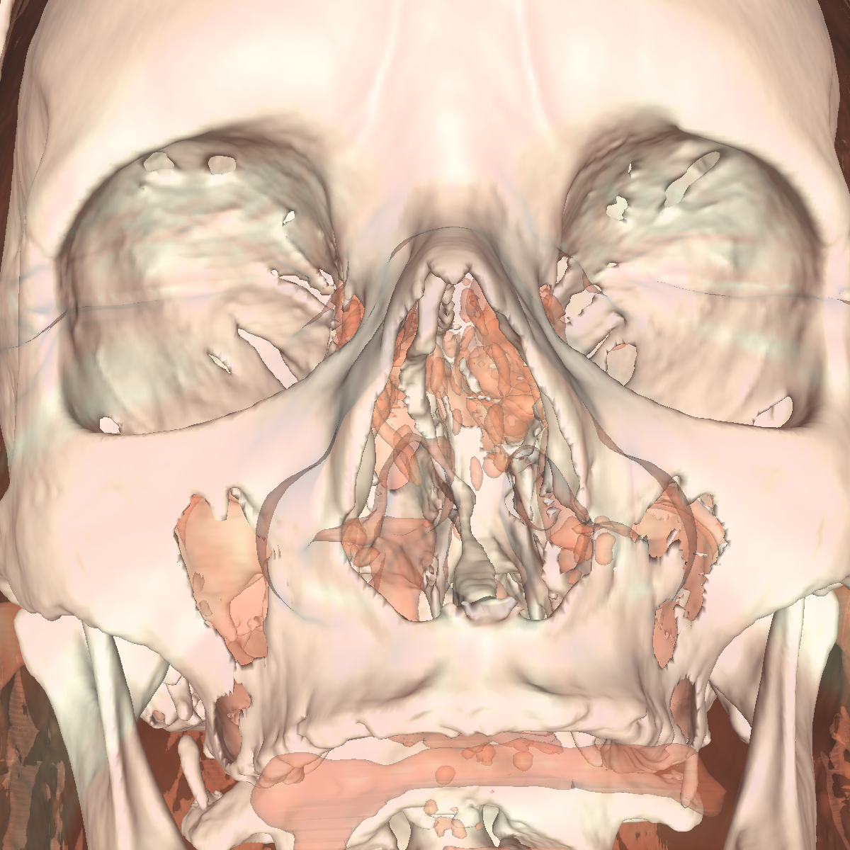
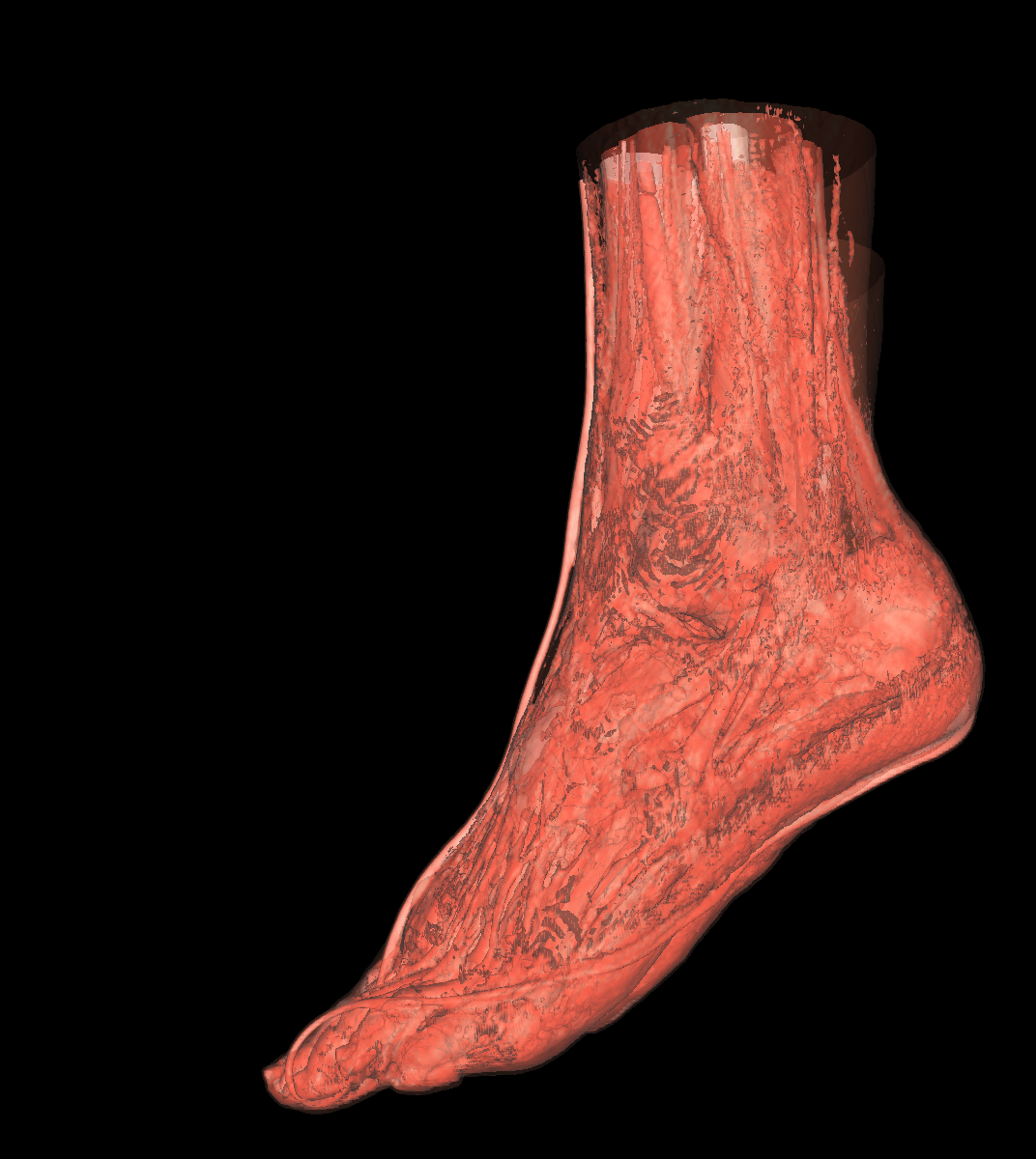
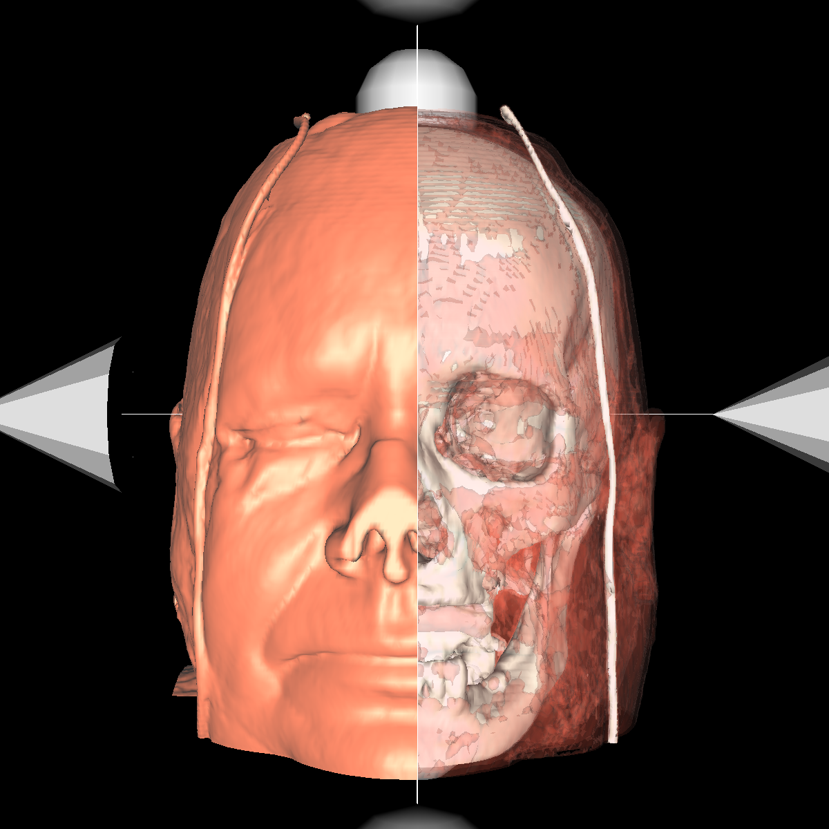
Part 3: Visualizing the Anatomical Structures using Transparency We visualize the anatomical structures creating an isosurface for each. Transparency is then applied to each isosurface revealing the multiple layers of anatomical structures. The outer structures/isosurfaces are assigned to be more transparent thus appropriately revealing the inner structures. We do this for both the feet and head datasets. We reuse our previous classification color map which allows for each anatomical structure to be differentiated from one another. We attempted to assign the tissue isosurface to have the greatest transparency difference between the other isosurfaces. We figured this would allow us to see more clearly features in the tissues/muscles. Therefore we used an opacity value of 0.30 for the skin (making it very highly transparent), 0.75 for the tissue isosurface, 0.85 for the bones, and 1.00 for everything above the bone threshold. For the feet, we set the opaqueness for the tissues to 0.50 since the tissues are more frequent structure in the feet. We have also tried other values as well such as making the skull/bones very transparent and assigning the tissues a higher opaqueness making them more visible. This allows the tissues to be seen more clearly with respect to the skull, but causes depth problems as some of the tissues covered by the nose/skull are now percieved to be infront of the skull. These screenshots are also shown below for reference. In the images below we can now clearly see multiple tissues and muscles in both the head and feet. Transparency is very useful to visualize nested interesting structures to gain a global perspective. It also is very useful to visualize muscles and tissues that would otherwise be very difficult to capture. The transparency adds perspective to these elements. |
Part 4: Extracting Interesting Features using Clipping We apply clipping which essentially intersects the volume/CT scan with a plane where everything on one side of the plane is removed allowing for the discovery of interesting features (i.e., these features would of otherwise been hidden). Clipping is also useful if you have a specific feature in mind and want to cut out the other parts of a visualization in order to get a better perspective. We found clipping to be useful in these ways, among others. We implemented clipping using an interactive on-screen GUI which can be either turned on or off by pressing 'i'. The GUI allows for the position and angle of the clipping plane to be dynamically changed by simply clicking on the pieces and moving your mouse in the direction in which you are changing. The clipping of the isosurfaces are particularly useful in viewing the brain (white matter) by clipping away pieces of the skull to expose the brain. Another use is to clip away unwanted tissues in order to see a tissue that is embedded close to the bone but would otherwise be blocked by other features. These ideas are shown in the various screenshots presented below. We have included clipping in the most general context using transparency combined with all the isosurfaces and also using simple single isosurfaces representing one specific anatomical structure. In the screenshots below we simply used the GUI to move around the position and angle of the clipping plane until we found an interesting region. For instance the most interesting feature is probably with respect to the evidence of the white matter by clipping the skull in various locations. These and other features are shown in the screenshots below. 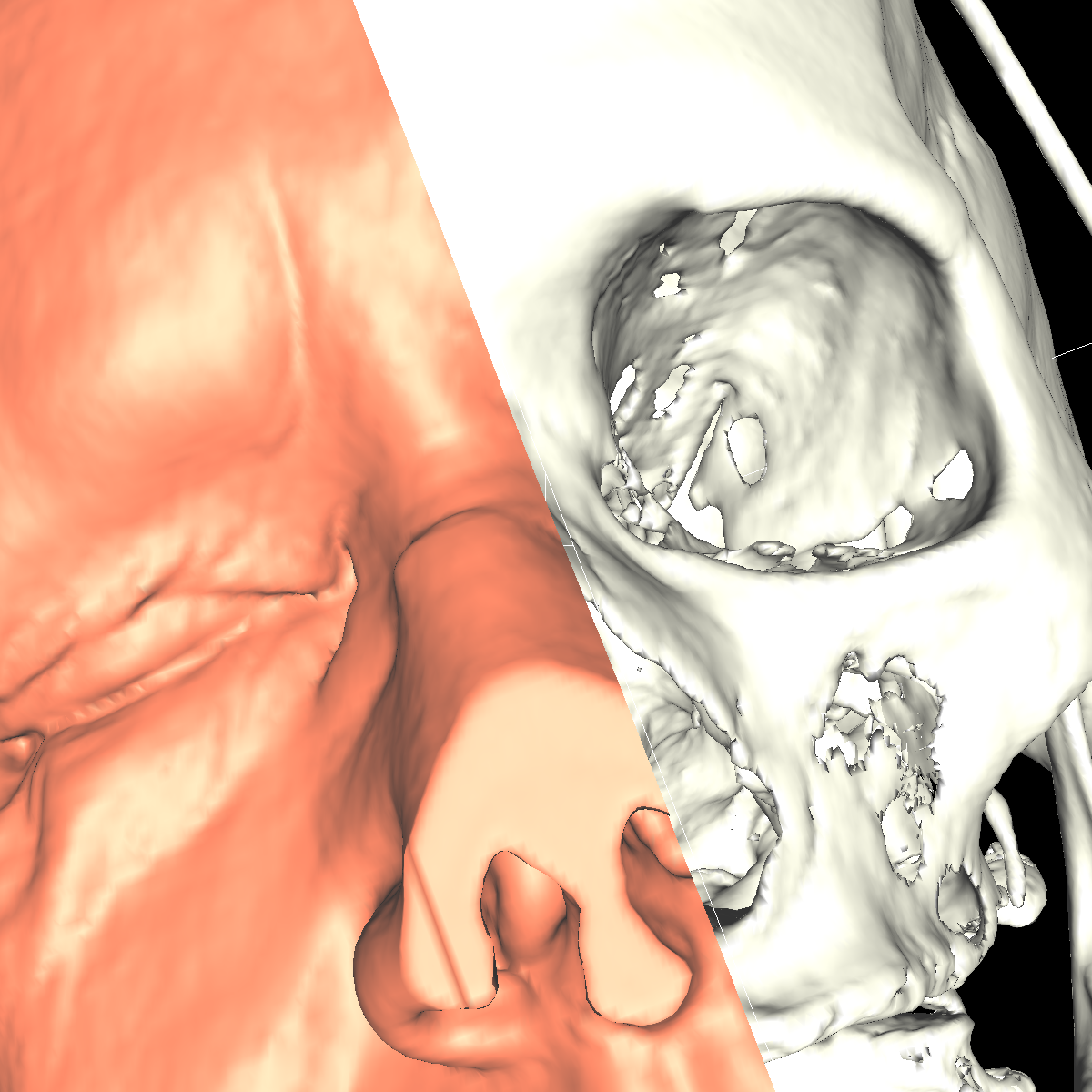 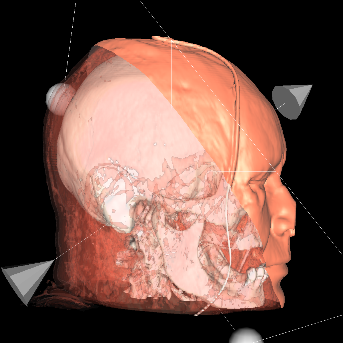 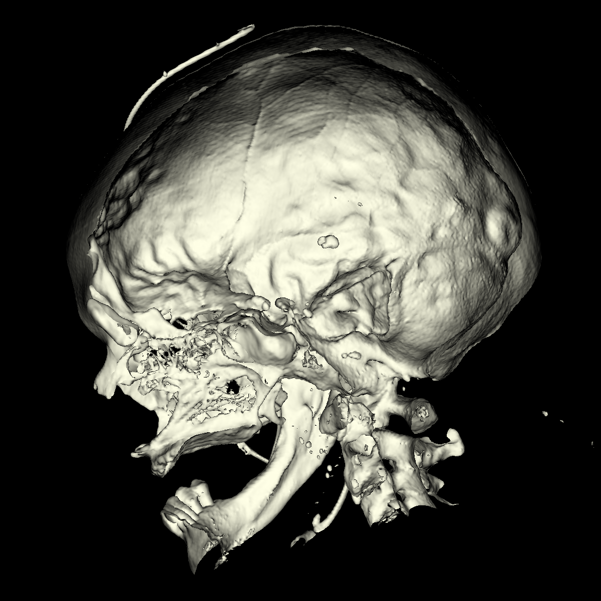 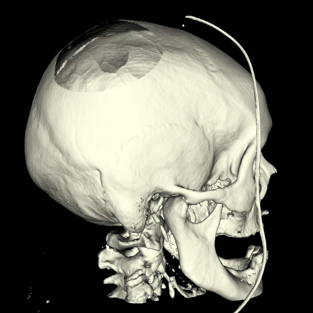 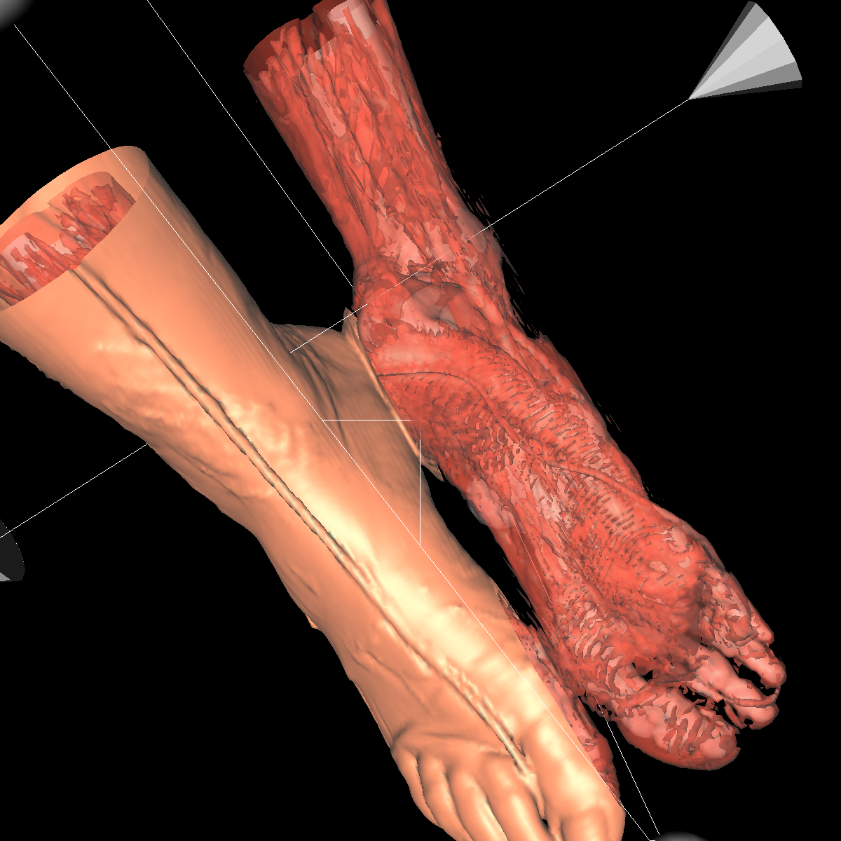  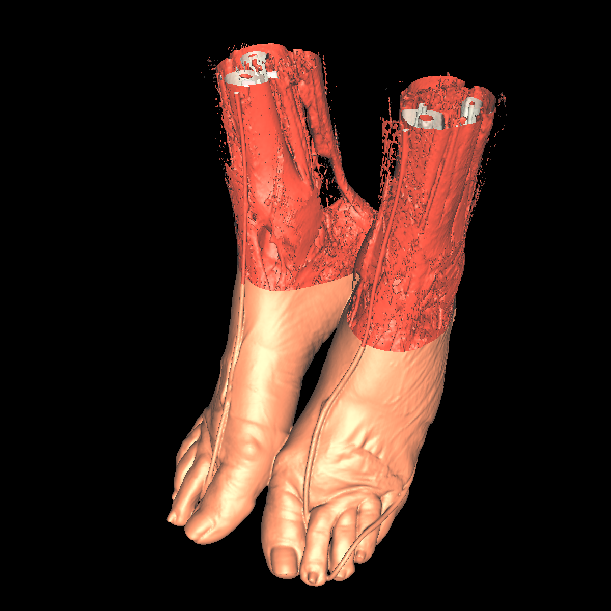 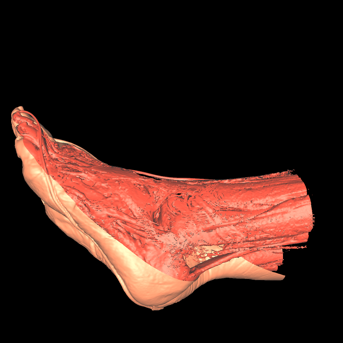 |
Discussion: Effectiveness of Isosurfaces for Medical Datasets Isosurfaces are an effective method to capture particular structures. Doctors and surgeons are often interested only in one specific feature of the scan and therefore clipping or simply finding the correct isovalue is highly effective. Compared to volume visualization, isosurfacing is also faster, though it has limitations if interested in seeing a complete view. The transparency is a solution to that problem, but the isosurfaces have to be explictly defined which is also a time consuming process and the resulting visualization suffers as compared to a pure volume visualization using ray-casting or other means. The transparency also allows us to see the tissue better. The clipping plane is another technique to cut away irrelevant pieces of the visualization in order to view an interesting feature more closely. However, there are a few short comings when using isosurfaces. For instance, if we are interested in tissue or other anatomical structures where the values osicilate then isosurfacing will fail to provide a good visualization. This is a problem even using clipping planes or other techniques. The other short coming seems to be the rendering speed as even the small datasets took a very long time to explore due to the necessary waiting after we changed the parameters of the visualization. This problem becomes even worse when we add multiple isosurfaces for each structure in which we are interested. This is probably not such a big deal if you have a system with a decent video card, but unfortunately most laptops seem to come standard with intergrated video cards. |
Other Experimental Visualizations In this section, we have included screenshots from other visualizations using the same dataset. More specifically, we created a very general GUI that allows for many different types of visualizations where multiple components can be applied collectively for the discovery of even more interesting features. 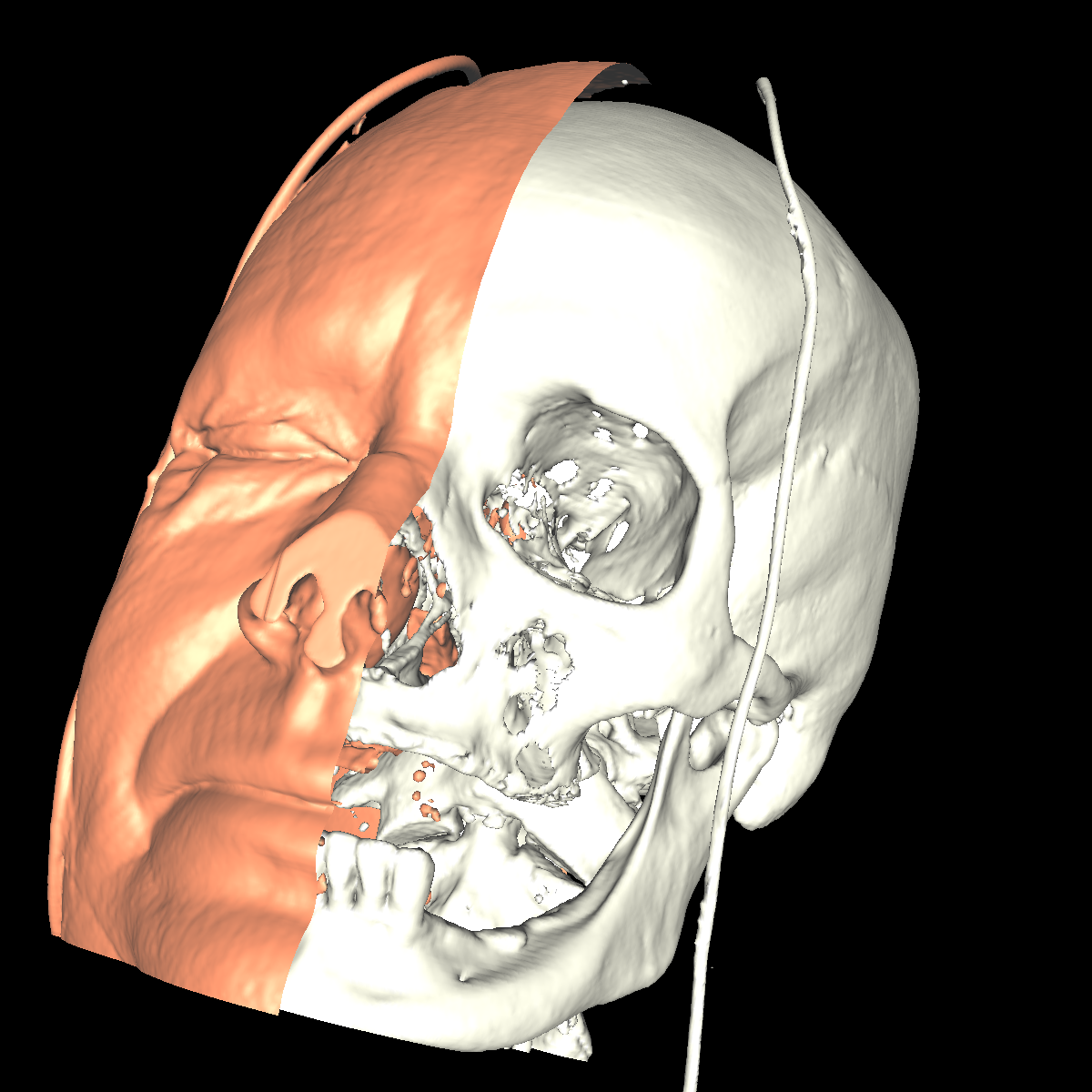

|